Chapter 3: Radar Signal Transmission and Reception
3.1 Transmitted Signals and Pulse Trains
Chapter 2 treated the echo as a time-varying signal: it has amplitude, frequency, can be sampled, and can be written in complex I/Q form. Within a radar system, this signal doesn't appear out of nowhere. The radar first transmits electromagnetic waves at a regular rhythm, these waves scatter off the target and return, then the receiver samples the weak returning voltage into data.
Looking at a single transmission, the receiver gets one echo record; transmitting continuously many times, these echo records stack up row by row into a matrix. Range processing, velocity processing, and detection all start from this matrix.
Pulse Radar Operation
Imagine you're in a dark cave and want to know if there's a wall ahead. You clap once, then hold your breath and listen for the echo. Hearing it means there's a wall; from how long the echo takes to return, you can estimate the distance. The speed of sound is approximately $340\,\text{m/s}$. If the echo returns after $0.6\,\text{s}$, the wall is roughly
away.
Pulse radar follows this same logic, just replacing sound waves with electromagnetic waves, and the speed changes from $340\,\text{m/s}$ to the speed of light $3\times10^8\,\text{m/s}$. The radar antenna first emits a very short electromagnetic pulse, then immediately stops transmitting, switches to receive mode, and waits for the echo reflected back from the target.
Converting the cave calculation to radar notation, if the echo is delayed by $\tau$ relative to the transmission time, the target range can be written as
The factor of $2$ in the denominator comes from the round-trip path: the electromagnetic wave travels from radar to target, then from target back to radar.
Pulse width is typically denoted $\tau_p$. If $\tau_p=1\,\mu\text{s}$, this pulse extends in space approximately
roughly several hundred meters in length. Pulse extension affects range resolution; for the receive window, after transmission ends, echoes from targets at different ranges return successively at different times.
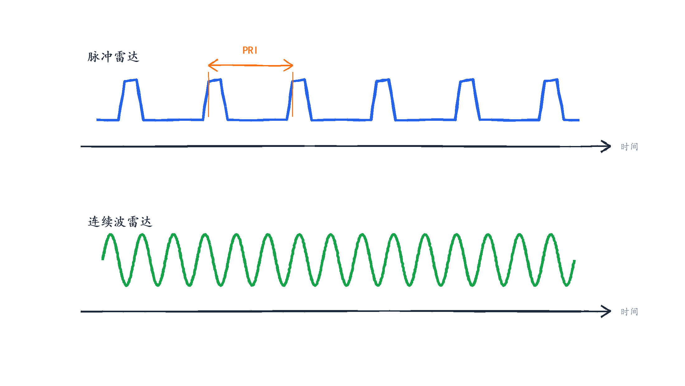
The upper portion of Figure 3.1 shows pulse radar: transmit for a short time, receive for the remaining time. The lower portion shows continuous wave radar: transmit continuously while also receiving continuously. Both approaches work for radar, but organize data differently.
PRI, PRF and Duty Cycle
Pulse radar doesn't transmit just one pulse. It transmits at regular intervals, forming a rhythmic pulse train. The time interval between the starting points of two adjacent pulses is calledPulse Repetition Interval(Pulse Repetition Interval, PRI). The reciprocal of PRI is calledPulse Repetition Frequency(Pulse Repetition Frequency,PRF):
For example, when PRI is $1\,\text{ms}$, PRF is $1000\,\text{Hz}$, meaning the radar transmits 1000 pulses per second.
PRI limits the maximum unambiguous range. If a distant target's echo hasn't yet returned before the radar transmits the next pulse, the receiver may not be able to distinguish whether this echo came from the previous pulse or from a nearby target after the new pulse. To avoid this confusion, the target echo's round-trip time must be less than PRI:
Therefore the maximum unambiguous range is approximately
When PRI is $1\,\text{ms}$, $R_{\max}=150\,\text{km}$. To see farther, you need to give distant echoes more return time, which means increasing PRI or decreasing PRF.
Another commonly used parameter isduty cycle(Duty Cycle), which represents the fraction of transmit time within the entire PRI:
If the pulse width $\tau_p=1\,\mu\text{s}$ and the PRI is $1\,\text{ms}$, the duty cycle is $0.1\%$. This means the radar spends most of its time receiving, with only a brief period transmitting. Average power may not be very high, but the peak power during pulse transmission can be substantial.
Continuous Wave Radar Operation
Continuous wave radar transmits continuously while receiving echoes simultaneously, eliminating the "transmit-then-listen" intervals. It is naturally suited for measuring Doppler frequency shifts because the transmitted signal is always present, allowing continuous observation of the echo's frequency offset relative to the transmitted signal. Speed guns are a typical example of continuous wave radar.
Continuous wave radar has difficulty measuring range because it lacks a clear "departure time." Frequency-modulated continuous wave (FMCW) radar addresses this by varying the transmit frequency over time, converting range information into beat frequency for processing. Many formulas commonly seen in automotive millimeter-wave radar originate from this approach.
Pulse radar provides the clearest decomposition of the "transmit, wait for return, then process" chain. Range, velocity, and detection problems can all be developed along this chain. The FMCW beat frequency formula represents a different way of organizing range information and follows a different data chain than pulse radar.
Pulse Trains and CPI
A single transmitted pulse yields one echo record. It can help measure range, but is insufficient for velocity and weak target detection.
Velocity information is typically reflected in phase changes between multiple echoes. If a target approaches the radar, each pulse return will have slightly more phase advance than the previous one; if the target recedes, the direction reverses. Observing only a single pulse makes it difficult to reliably determine this pulse-to-pulse change.
Weak targets also require multiple observations to accumulate evidence. A single echo may be buried in noise, but when dozens or hundreds of consecutive echoes are combined, the target response becomes easier to extract from the background.
Therefore, radar processing typically operates on a burst of pulses. This burst of pulses used for joint processing corresponds to aCoherent Processing Interval(Coherent Processing Interval, CPI). "Coherent" indicates that these pulses maintain a stable phase relationship, making pulse-to-pulse comparisons meaningful. If a CPI contains $N_p$ pulses with PRI $T_r$, the CPI duration is approximately
Here, think of the CPI as an observation period composed of multiple transmitted pulses. Chapter 5 on velocity processing will formally use this concept.
3.2 Target Reflection and Point Target Model
Target Scattering of Electromagnetic Waves
What happens when electromagnetic waves transmitted by a radar encounter aircraft, ships, raindrops, terrain, or buildings?
The answer is somewhat surprising: they don't simply "bounce straight back," nor do they "pass through completely." The reality is closer to scattering: different locations on the target surface redirect energy in different directions, with only a portion returning to the radar antenna.
Think about it: when you shout into a valley, the mountain gives you an echo; a fly will also scatter a tiny bit of energy, but it's negligible. If flies could produce clear echoes, life would be quite chaotic. When radar observes targets, it's essentially dealing with this question of "who can send energy back, and how much."
When a mirror reflects visible light, energy returns primarily in a specific direction; aircraft or ship surfaces have complex shapes, and metal edges, curved surfaces, gaps, and coatings all affect how electromagnetic waves scatter. A slight change in target orientation can significantly alter the echo strength observed by the radar.
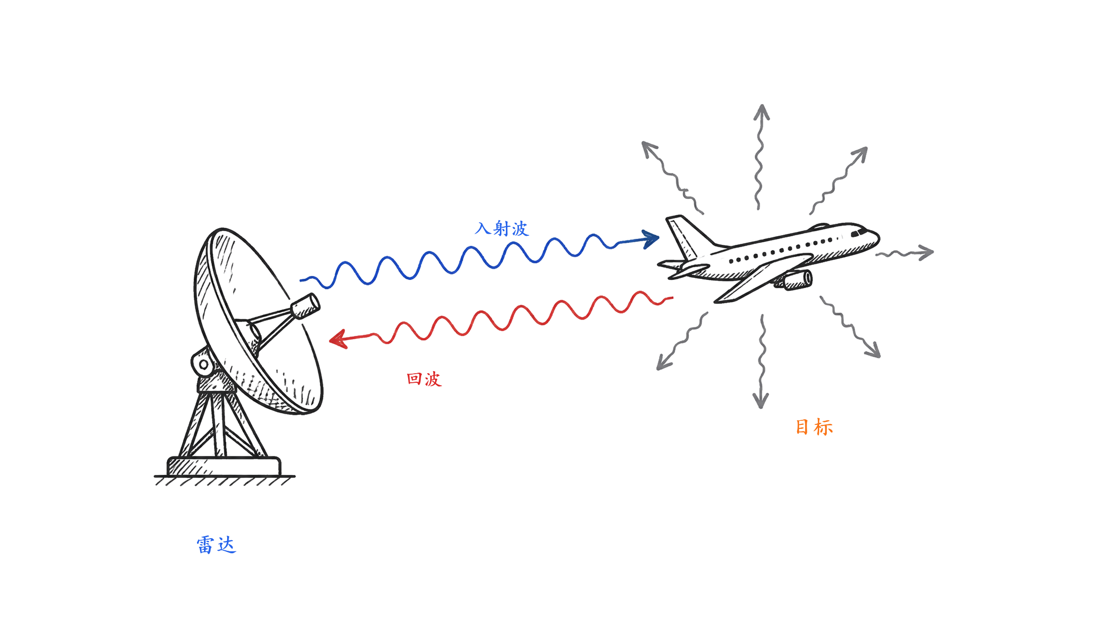
In Figure 3.2, the incident wave scatters in multiple directions after striking the target. The radar only receives the small fraction of energy that returns along the echo direction. Stealth shaping and radar-absorbing materials primarily work by reducing the energy returned toward the radar direction.
When I was a child, I heard about stealth fighters and thought the aircraft were literally invisible to the naked eye. Now I know that 'stealth' here refers more to being invisible to radar.
Radar Cross Section (RCS)
Engineers need a number to describe 'how bright a target appears to radar.' This number is calledRadar Cross Section(Radar Cross Section, RCS), typically denoted as $\sigma$, with units of square meters.
The definition of RCS is somewhat convoluted. Its unit is square meters, but you should never think of it as the target actually having a physical area of that size. It's more like asking: how'bright' does this target appear to the radar? If an ideal target could produce an echo as strong as the real target, we use the equivalent area of that ideal target to represent the scattering capability of the real target. If it can only reflect half the energy, the equivalent area becomes correspondingly smaller; this example isn't rigorous, but it helps you grasp the word 'equivalent.' The larger the RCS, the stronger the received echo is typically at the same distance and radar parameters.
An aircraft may have large physical dimensions, but if its shape and materials deflect most of the energy away from the radar direction, its RCS can be very small. A thin, elongated metal rod has a small geometric cross-sectional area, but at certain angles it may also produce strong reflections. RCS measures the 'ability to scatter back toward the radar direction,' not how much space the target occupies.
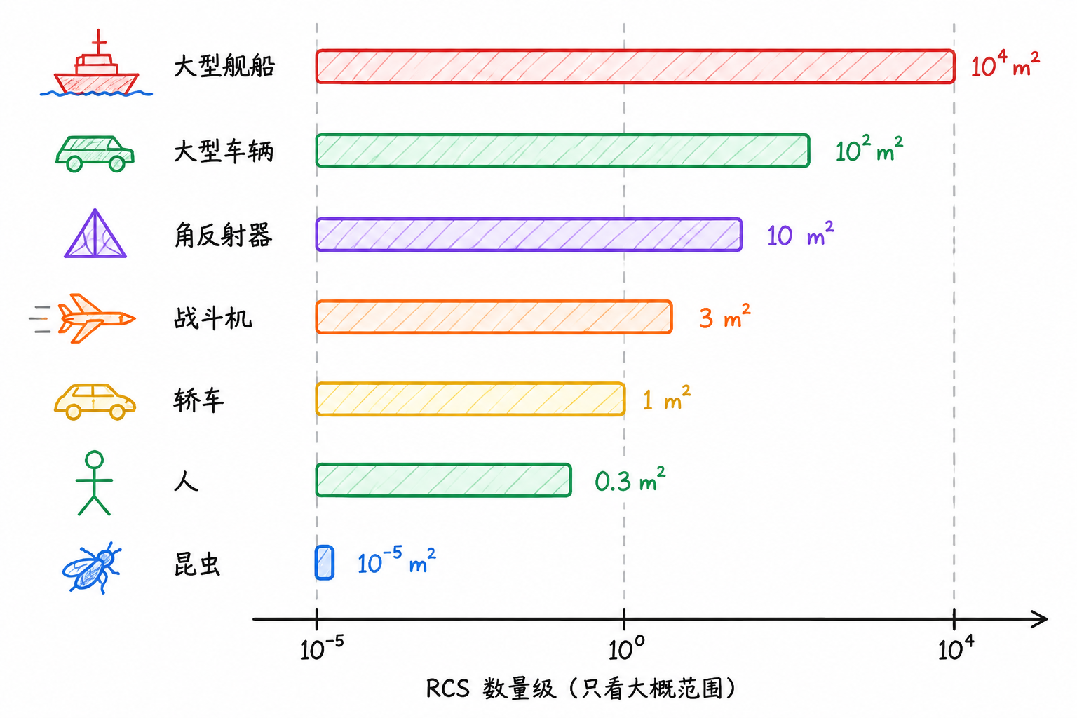
Figure 3.3 uses a logarithmic scale to show the order-of-magnitude differences in RCS for various targets. From insects to large ships, RCS can span many orders of magnitude. This difference affects echo power and also impacts subsequent detection difficulty.
RCS also varies with observation angle and frequency. The same aircraft may have very different RCS when facing the radar head-on versus from the side; the same target may exhibit different scattering characteristics at meter-wave, centimeter-wave, and millimeter-wave frequencies. The details of electromagnetic scattering serve as a reminder here: RCS is an engineering estimate, not a fixed geometric constant. Engineering calculations must account for this variability and handle it through measurement, calibration, and margin design.
Point Target Assumption
Real targets have size and shape, and may consist of multiple scattering points. An aircraft has a nose, wings, tail, and engines; a ship has masts, decks, and hull sides; the echoes from these parts may have different delays and phases.
If we really accounted for an aircraft's nose, wings, engines, and edge gaps, this chapter would turn into an electromagnetic scattering course. We'll start with a very useful simplification: treat the target as apoint target. A point target does not require the target to actually have no size; it means that under the current radar resolution capability, the target can be collapsed into an equivalent response at a single location.
In the simplified model of this book, a point target is primarily described by three quantities:
| Quantity | What it determines | Manifestation in the echo |
|---|---|---|
| Range $R$ | Round-trip propagation time | Echo delay $\tau=2R/c$ |
| Radial velocity $v_r$ | Target motion along the radar line of sight | Doppler shift $f_d=2v_r/\lambda$ |
| RCS $\sigma$ | Target's ability to scatter energy back toward the radar | Echo amplitude magnitude |
The point target assumption simplifies subsequent processing: the target's shape is set aside for now. First, use delay to find range, use interpulse phase or frequency change to find velocity, then determine whether this response is reliable against the background. When it comes to high-resolution imaging and complex target scattering, those details can be brought back in.
3.3 Range Attenuation and Radar Equation
Shout in a valley, and the nearby cliff echoes loudly while the distant peak echoes faintly. As sound waves propagate, energy spreads over the spherical surface area, resulting in attenuation on the order of $1/R^2$. Radar echoes travel a round-trip path: first from the radar to the target, then from the target back to the radar, experiencing two expansions. The received power attenuates as $1/R^4$. When the target distance doubles, the received power becomes $1/16$ of the original.
This fourth power comes from two legs.
Outbound $1/R^2$
First consider the energy transmitted by the radar. Assume the transmit power is $P_t$, and temporarily treat the antenna as radiating uniformly in all directions. When the electromagnetic wave propagates to distance $R$, the transmit power has spread over a spherical surface of radius $R$ with area $4\pi R^2$.
The power density at the target is
Real radar antennas have directionality, concentrating energy in a particular direction. Using antenna gain $G$ to represent this concentrating capability, the power density in the main direction can be written as
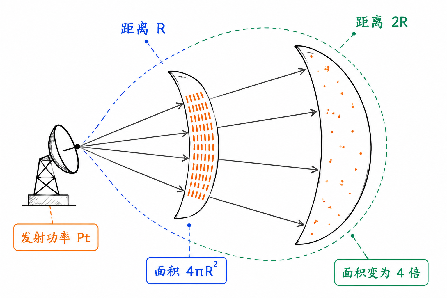
This is the first $R^2$. It comes from energy spreading over the spherical surface area.
Return $1/R^2$
After the target is illuminated by power density $S_1$, it scatters part of the energy back toward the radar. The role of RCS $\sigma$ in the radar equation is to equate the complex scattering process of a real target into "how much echo can be produced in the radar direction." RCS does not mean the target actually intercepts a geometric area of a flat plate with area $\sigma$; it is an equivalent quantity defined by echo strength.
Using this equivalent quantity, the scattered power density in the radar direction can be written as
The $4\pi R^2$ in the denominator represents the echo spreading again over the spherical surface area as it returns to the radar. Substituting the outbound power density gives
One $R^2$ on the outbound leg, one $R^2$ on the return leg, combined to give $R^4$.
Received Power Equation
The radar receiving antenna cannot collect energy from the entire spherical surface, only the small portion covered by the effective aperture. The effective aperture of the receiving antenna is denoted $A_e$, and the received power is
There is a relationship between effective aperture and antenna gain
where $\lambda$ is the operating wavelength. Substituting this gives the basic radar equation commonly seen for monostatic radar:
If transmit and receive antenna gains differ, it can also be written as $G_tG_r$. Most simplified examples in this book assume transmit and receive share the same antenna, so it's written as $G^2$.
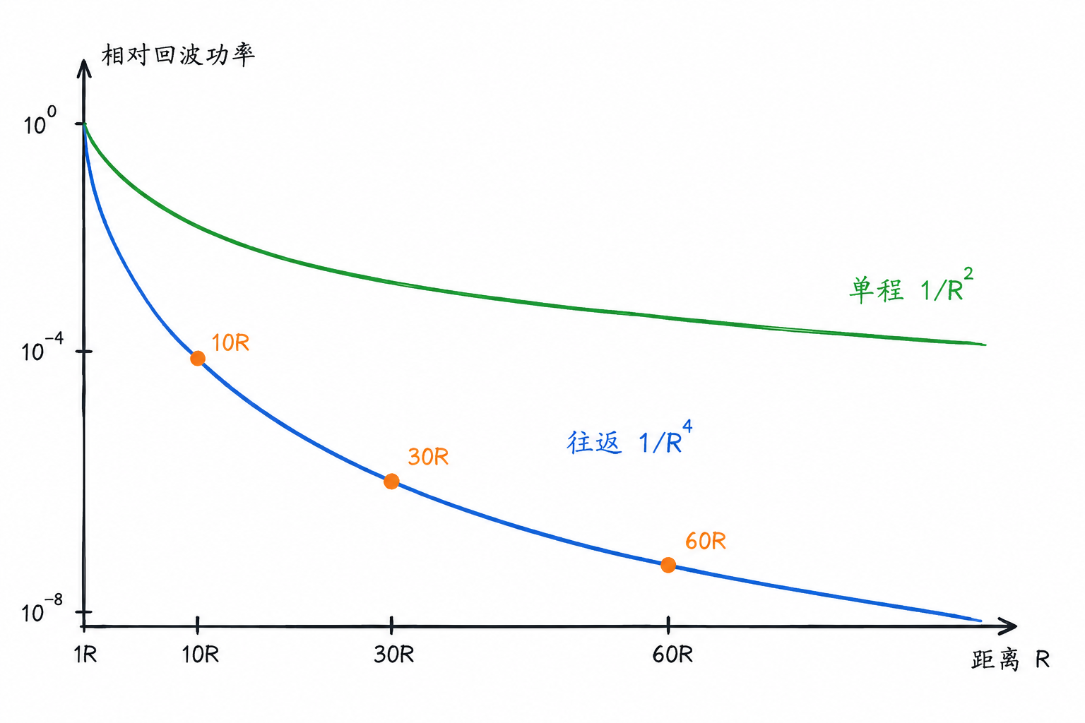
Figure 3.5 plots both $1/R^2$ and $1/R^4$. Radar echo undergoes spreading in both the outbound and return paths, attenuating faster than single-path propagation. When range increases from $50\,\text{km}$ to $100\,\text{km}$, received power drops to $1/16$; from $100\,\text{km}$ to $200\,\text{km}$, it drops to $1/16$ again.
The radar equation also provides engineering insights. Increasing transmit power $P_t$ strengthens the echo; increasing antenna gain $G$ benefits both transmit and receive; larger target RCS $\sigma$ makes detection easier; range $R$ is the hardest parameter to overcome because it appears as a fourth power in the denominator.
Real systems must also account for atmospheric absorption, rain attenuation, feedline losses, system noise, ground multipath, and other factors. Grasping the main structure is sufficient for now: long-range radar is challenging not only because targets are far, but more critically because the echo must travel a round-trip path, causing extremely rapid power attenuation.
This article breaks down $1/R^4$: radar echo must travel both outbound and return paths.
3.4 Receiver Signal Model
Time Delay, Amplitude Attenuation, and Doppler
We've examined transmission, scattering, and range attenuation separately. Combining them, a point target echo can be viewed as the transmitted signal after three types of changes: slightly delayed, significantly weakened, and with minor frequency or phase variations.
Time delay is determined by range:
A target at $150\,\text{km}$ corresponds to a round-trip delay of
Echoes from long-range targets are often extremely weak, requiring receiver amplification and subsequent processing to be detectable.
If the target moves along the radar line of sight, the echo frequency will exhibit Doppler shift. In monostatic radar, this is commonly written as
where $v_r$ is theradial velocity, i.e., the component of target velocity along the radar line of sight. By convention, approaching the radar is positive, receding is negative.
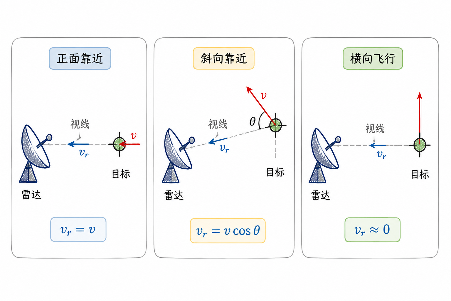
Figure 3.6 illustrates three scenarios. When the target approaches head-on, radial velocity equals target velocity and Doppler shift is maximum; when approaching at an angle, only the velocity component along the line of sight is used; when passing tangentially, radial velocity approaches zero and Doppler shift is also near zero. Radar sees 'approaching or receding' through Doppler, not the target's complete motion.
Consider a numerical example. An X-band radar operates at wavelength $\lambda=3\,\text{cm}$, and a target approaches with radial velocity $100\,\text{m/s}$, then
Compared to a carrier frequency on the order of $10\,\text{GHz}$, a shift of several kilohertz is small; however, it can be reliably measured in the frequency domain or across pulse phases.
If written in complex baseband form, the echo from a single point target can be simplified to
Here $s(t)$ is the transmitted signal, $\tau$ represents delay, $\alpha$ is the complex amplitude incorporating propagation loss, RCS, and initial phase, $f_d$ represents Doppler shift, and $w(t)$ represents noise. This equation ties together the preceding concepts: range becomes delay, RCS and range attenuation become amplitude, and velocity becomes Doppler.
Noise, Clutter, and Interference
The receiver does not only capture target echoes. Real data also contains noise, clutter, and interference. All three make targets harder to detect, but they have different origins.
| Component | Source | Impact on Subsequent Processing |
|---|---|---|
| Noise | Random disturbances such as receiver thermal noise and quantization noise | Raises the noise floor and reduces SNR |
| Clutter | Environmental echoes from ground, sea surface, rain, buildings, etc. | May be stronger than targets, often concentrated in specific range or Doppler regions |
| Interference | Other radars, communication signals, transmitter leakage, or intentional jamming | May appear as strong narrowband, wideband, or non-stationary components |
Noise can be described by its power. Receiver thermal noise is commonly written as
where $k$ is Boltzmann's constant, $T$ is the system temperature, $B$ is the receiver bandwidth, and $F$ is the noise figure. Wider bandwidth typically means more received noise.
Clutter can be understood as real echoes produced by the environment, typically from sources that are not the targets of interest. Ground, sea surface, and rain can all reflect electromagnetic waves. Both fixed thresholds and CFAR must contend with this background variation.
Interference is more like energy intruding from outside or within the system. It may come from nearby radars or from transmitter leakage. The distinction is straightforward: noise is random background, clutter is environmental echoes, and interference is external or leakage signals.
This article models point-target echoes as signals jointly affected by delay, attenuation, and Doppler.
3.5 From I/Q Samples to Echo Matrix
From RF Echo to I/Q Samples
The antenna receives a high-frequency analog voltage. For example, an X-band radar may have a carrier frequency near $10\,\text{GHz}$. What the computer ultimately processes is a sequence of complex samples, not the $10\,\text{GHz}$ waveform itself. The receiver circuitry in between is complex, but by the time it reaches the algorithm input, the form has converged to a set of I/Q digital samples.
The receiver downconverts the RF echo to a lower frequency, or to near baseband, then converts it into I/Q digital samples. As seen in Chapter 2, I/Q can form complex samples.
A complex sample stores both amplitude and phase. Amplitude is used to determine echo strength, while phase is used for subsequent velocity processing.
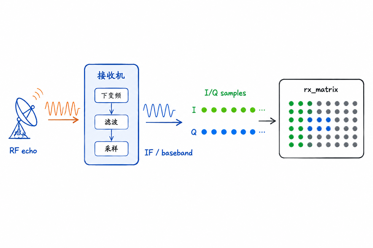
Figure 3.8 illustrates the data transformation: at the antenna side is a high-frequency analog echo, which the receiver downconverts to IF or near baseband, then samples into I and Q digital channels. Each transmitted pulse yields a sequence of complex I/Q samples, and multiple pulses are arranged by transmit order, commonly denoted in code as rx_matrix。
The following table lists this data transformation.
| Stage | Data form | Role in algorithm |
|---|---|---|
| RF echo | High-frequency analog echo received by antenna | Generally not directly processed by computer |
| IF / baseband | IF or baseband signal after downconversion | Preserves echo amplitude and phase |
| complex I/Q samples | Discrete complex sequence $x[n]=I[n]+jQ[n]$ | Serves as signal processing input |
rx_matrix | I/Q sample matrix from multiple transmitted pulses | Range and velocity processing begins here |
The terms dechirp, beat frequency, and range FFT found in FMCW literature belong to frequency-modulated continuous-wave radar data organization. They are not part of the same data chain as the pulse echo matrix in this section, and the beat frequency formula does not apply here.
One Transmitted Pulse Corresponds to One Fast-Time Sequence
After the radar transmits a pulse, the receiver samples continuously for a period of time. Assuming a sampling rate of $f_s$, the sampling interval is
Use a set of small numbers to familiarize with the notation of $\mathbf r_0$. Assuming the receiver samples at $f_s=10\,\text{MHz}$, then $T_s=0.1\,\mu\text{s}$. If the receive window takes the first 8 samples after one transmitted pulse, a complex sequence is obtained:
| Notation | Reading convention |
|---|---|
| $r_0[0]$ | The 0th sample point in the 0th transmitted pulse |
| $r_0[1]$ | The 1st sample point in the 0th transmitted pulse |
| $r_0[4]$ | The 4th sample point in the 0th transmitted pulse |
| $r_0[7]$ | The 7th sample point in the 0th transmitted pulse |
The subscript $0$ in $r_0$ indicates the 0th transmitted pulse, and the $n$ in brackets indicates the sample index within that pulse. If we want to mark the time for the $n$th sample point, it is
Therefore, within a single pulse there is a very short sampling time axis. The sampling time within this pulse is commonly calledfast time(fast time). It changes very rapidly, typically on the order of nanoseconds to microseconds. Chapter 4 will search for echo delays along this dimension; here, we first treat $\mathbf r_0$ as 'a row of complex samples acquired from a single pulse.'
Formed by multiple pulses rx_matrix
Now repeat the 'single row of data' from the previous subsection multiple times. Using the same example, if 4 pulses are transmitted within a CPI, with 8 sample points acquired for each, then the 0th, 1st, 2nd, and 3rd transmissions yield four sequences:
Arranging them row by row in transmission order gives a $4\times 8$ rx_matrix:
| pulse/sample | $n=0$ | $n=1$ | $n=2$ | $n=3$ | $n=4$ | $n=5$ | $n=6$ | $n=7$ |
|---|---|---|---|---|---|---|---|---|
| $m=0$ | $r_0[0]$ | $r_0[1]$ | $r_0[2]$ | $r_0[3]$ | $r_0[4]$ | $r_0[5]$ | $r_0[6]$ | $r_0[7]$ |
| $m=1$ | $r_1[0]$ | $r_1[1]$ | $r_1[2]$ | $r_1[3]$ | $r_1[4]$ | $r_1[5]$ | $r_1[6]$ | $r_1[7]$ |
| $m=2$ | $r_2[0]$ | $r_2[1]$ | $r_2[2]$ | $r_2[3]$ | $r_2[4]$ | $r_2[5]$ | $r_2[6]$ | $r_2[7]$ |
| $m=3$ | $r_3[0]$ | $r_3[1]$ | $r_3[2]$ | $r_3[3]$ | $r_3[4]$ | $r_3[5]$ | $r_3[6]$ | $r_3[7]$ |
For example, the cell $r_2[4]$ represents 'the sample point with index $n=4$ in the pulse numbered $m=2$.' Reading horizontally across a row gives the fast-time sequence acquired from a single pulse; reading vertically down a column gives samples at the same sampling position across different pulses.
In general form, a CPI contains $N_p$ transmitted pulses, with $N_s$ sample points acquired per pulse, forming the matrix
In code, this can be called rx_matrix. Its dimensions are
where $N_p$ is the number of pulses and $N_s$ is the number of sample points per pulse. That is, the number of rows equals the number of pulses, and the number of columns equals the number of sample points per pulse.
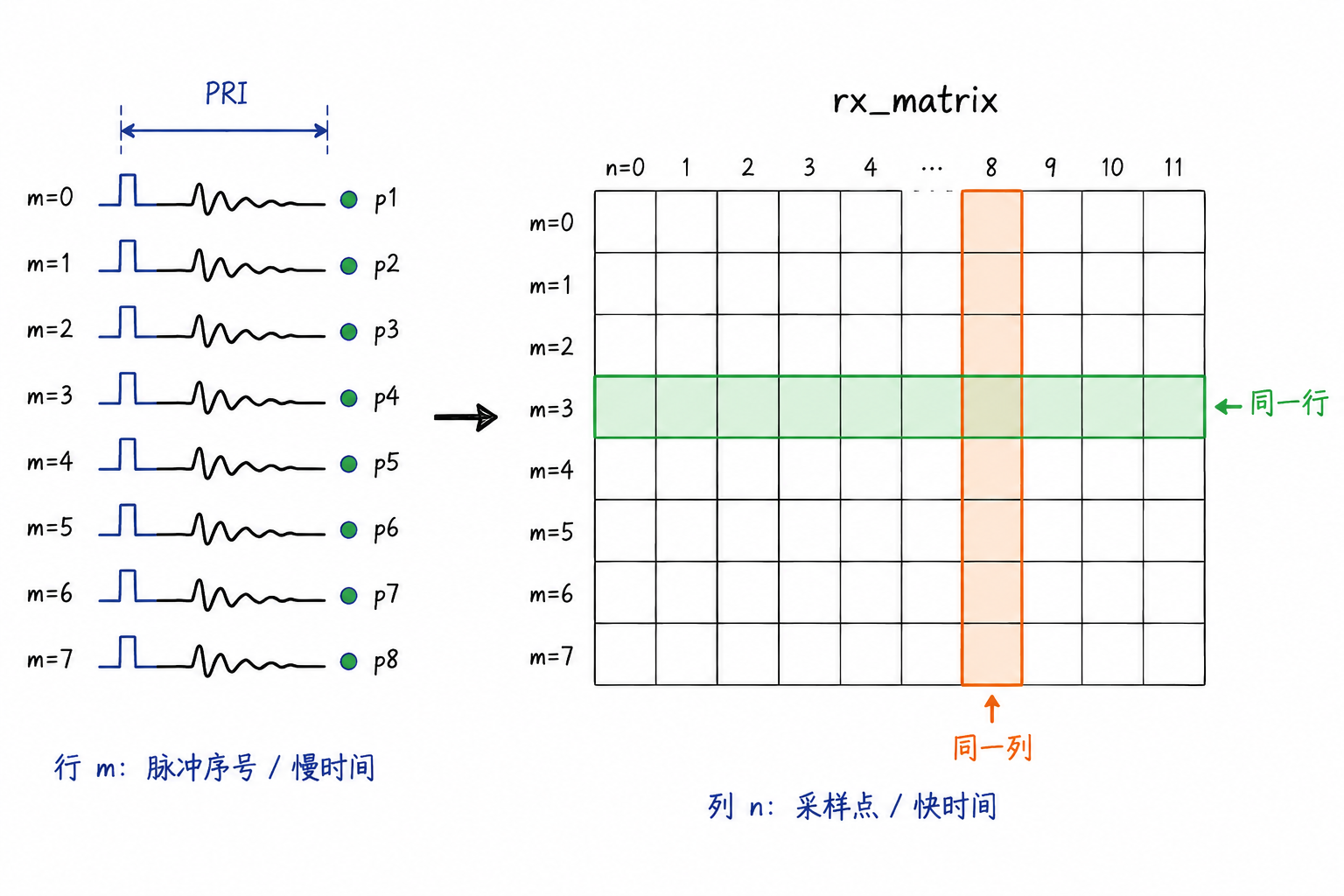
In Figure 3.9, the column direction is fast time: within the same row, from left to right, the column index $n$ increases, corresponding to echo delays from near to far. The row direction is slow time: the row index $m$ increases from top to bottom, corresponding to the $m$th transmitted pulse. Adjacent rows are separated by one PRI.
Fast time is used to find range, while slow time is used to compare phase changes between multiple pulses. If a stationary target remains at approximately the same range, it will repeatedly appear near the same column; for a moving target, not only may its range change, but its complex phase will also gradually rotate from row to row. Chapter 4 finds delay and range along the column direction, while Chapter 5 examines phase changes and velocity along the row direction.
This article clearly explains the rows and columns of rx_matrix : columns correspond to fast time, rows correspond to slow time.
3.6 Exercises
Exercise 1: Round-Trip Time and Range
A pulse radar receives an echo from a target and measures the echo delay relative to the transmission time as
(a) How far is the target from the radar?
(b) If this radar has a PRI of $1\,\text{ms}$, what is the maximum unambiguous range? Does this target exceed the maximum unambiguous range?
Solution: The target range is determined by the round-trip time:
The maximum unambiguous range is
The target range is $60\,\text{km}$, which does not exceed the maximum unambiguous range.
Exercise 2: PRI, PRF, and Duty Cycle
A radar has a PRI of $2\,\text{ms}$ and a pulse width of $2\,\mu\text{s}$.
(a) What is the PRF?
(b) What is the duty cycle?
(c) If the average transmit power is $1\,\text{kW}$, what is the approximate peak power?
Solution: The PRF is
The duty cycle is
The average power and peak power approximately satisfy
Therefore
Although the average power of pulse radar may not appear high, the peak power at the moment of transmission can be very large.
Exercise 3: Understanding the Magnitude of Range Attenuation
Two targets have the same RCS and all other conditions are identical. Target A is $50\,\text{km}$ from the radar, and target B is $100\,\text{km}$ from the radar.
(a) What fraction of target A's received power does target B have?
(b) If target A's SNR is $30\,\text{dB}$, what is target B's SNR approximately?
Solution: Received power is proportional to $1/R^4$. Target B is at twice the range of target A, so the received power becomes
A power drop of $1/16$ corresponds to a dB change of
If noise power remains constant, SNR also drops by about $12\,\text{dB}$, from $30\,\text{dB}$ to approximately $18\,\text{dB}$.
Exercise 4: Doppler Frequency Shift Calculation
An S-band radar operates at wavelength $\lambda=0.1\,\text{m}$. A target approaches the radar with radial velocity $v_r=200\,\text{m/s}$.
(a) What is the Doppler shift $f_d$?
(b) If the target flies tangentially at the same speed with radial velocity approximately 0, what happens to the Doppler shift?
Solution: When approaching
If the target flies tangentially, the radial velocity approaches 0, so
This shows that Doppler shift only reflects target motion along the radar line of sight.
Exercise 5:rx_matrix dimensions
A radar transmits $64$ pulses in one CPI. The receive window after each pulse samples $1024$ complex I/Q points.
(a)rx_matrix What are the dimensions?
(b) Which dimension corresponds to fast time? Which dimension corresponds to slow time?
(c) In which direction does Chapter 4 range processing primarily operate? In which direction does Chapter 5 velocity processing primarily operate?
Solution: Each pulse produces a fast-time sequence of length $1024$, and there are $64$ pulses in total. Therefore the matrix dimensions are
The row direction corresponds to pulse number, i.e., slow time; the column direction corresponds to in-pulse sample points, i.e., fast time.
Chapter 4 range processing primarily operates along the column direction to find echo delays; Chapter 5 velocity processing primarily operates along the row direction to compare phase changes across multiple pulses.