Chapter 2: Signal Fundamentals

2.1 What is a Signal

Chapter 1 explained how radar can extract target information from echoes. What a real receiver first obtains is a voltage curve that fluctuates over time; range, velocity, and detection results must all be calculated from this curve.

This chapter teaches you how to read this curve: how to describe amplitude and frequency, how to interpret spectra, what information sampling loses, and why radar data is often represented as complex I/Q.

Signals and Sine Waves

The voltage curve recorded by a radar receiver is a signal. A thermometer reading is a single number, but a record of temperature changing over time is a signal. What signals have in common is: the value changes continuously, and the change itself carries information.

The most commonly used signal form in engineering is the sine wave. Let's start with the simplest notation:

s(t) = A \sin(2\pi f t)

The formula has two parameters:amplitude $A$ andfrequency $f$. The $2\pi$ comes from "one complete cycle corresponds to $2\pi$ radians," so $2\pi f t$ represents the total phase accumulated in $t$ seconds.

Amplitude $A$ describes the signal strength, i.e., the maximum distance the waveform deviates from zero, typically measured in volts (V). Under the same conditions, a larger amplitude usually means a stronger signal.

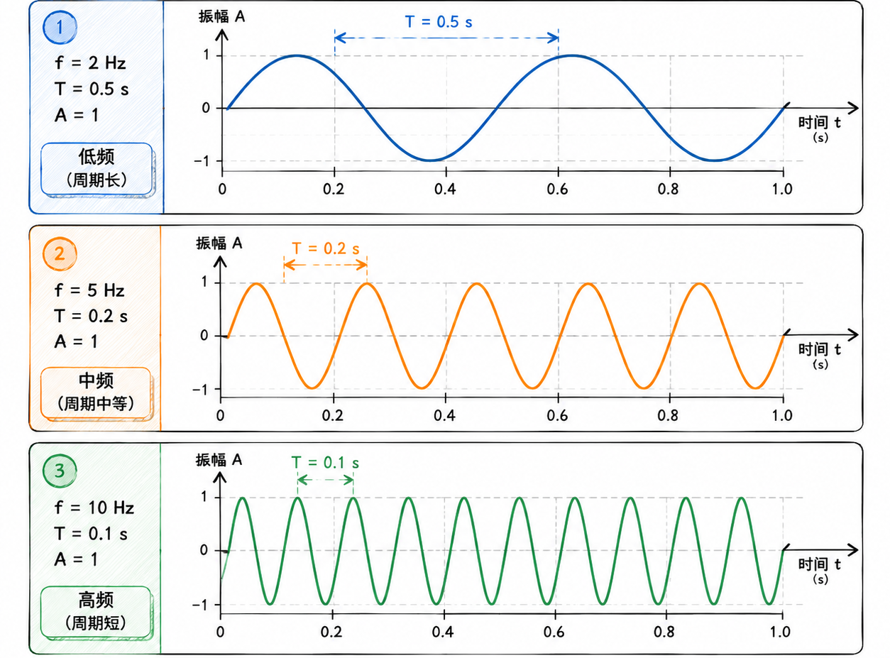
Frequency $f$ describes how many complete oscillations occur per second, measured in hertz (Hz). The reciprocal of frequency is theperiod $T = 1/f$, which represents the time required to complete one full oscillation.

Figure 2.1 shows three sine waves at 2 Hz, 5 Hz, and 10 Hz. The 2 Hz waveform completes only two oscillations in 1 second, with period $T = 0.5$ s, appearing smooth. The 10 Hz wave packs 10 oscillations into the same 1 second, appearing much denser. Higher frequency means more oscillations "packed into" the same time interval.

Figure 2.1 Sine waves at three frequencies

Frequency and Wavelength

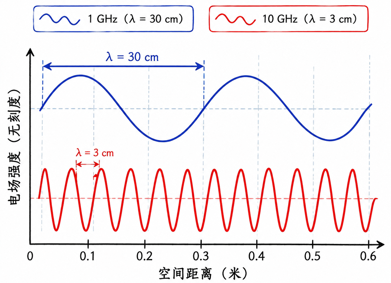
When electromagnetic waves propagate through space, the distance between adjacent peaks is called thewavelength $\lambda$, which relates to frequency by:

\lambda = \frac{c}{f}

$c \approx 3\times10^8$ m/s is the speed of light. Frequency describes how many oscillations occur per second, while wavelength describes the spatial distance between adjacent peaks; higher frequency means shorter wavelength. Figure 2.2 illustrates this spatial distance.

Figure 2.2 Electromagnetic wave wavelength diagram

Wavelength will appear in velocity formulas later. When a target moves, the echo frequency shifts slightly, and radar can use this frequency difference to measure velocity.

Composite Signals

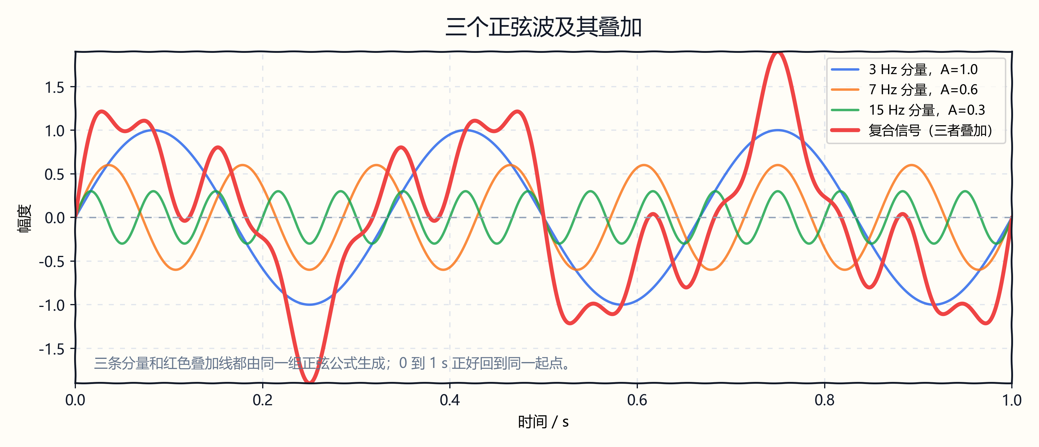
Real echoes are rarely single sine waves and often contain multiple frequency components. Let's start with a simplified example using three sine waves.

Figure 2.3 plots three sine waves together: 3 Hz (amplitude 1.0), 7 Hz (amplitude 0.6), and 15 Hz (amplitude 0.3). The three thin lines are the individual components, and the thick red line is their composite signal. The composite signal fluctuates irregularly, and it's nearly impossible to guess by eye alone that it's composed of three frequencies.

Figure 2.3 Three sine waves and their superposition

A radar echo can first be read as a signal that varies with time: amplitude, frequency, and wavelength are the most fundamental readings.

2.2 Time Domain and Frequency Domain

The same signal can be described in two ways.

Time Domainis the most familiar perspective: the horizontal axis is time, the vertical axis is the signal value. Electrocardiograms, audio waveforms, curves on an oscilloscope screen—all are time-domain representations.

Frequency Domaintakes a different angle: the horizontal axis is frequency, the vertical axis is the intensity of that frequency component. It shows which frequencies are present in the signal and their relative proportions.

Which perspective to choose depends on what question you want to answer. If you want to know the voltage at a particular moment, look at the time domain; if you want to know which frequencies are mixed in the signal, look at the frequency domain.

Time Domain and Frequency Domain

The four-panel figure below shows the correspondence between time domain and frequency domain side by side.

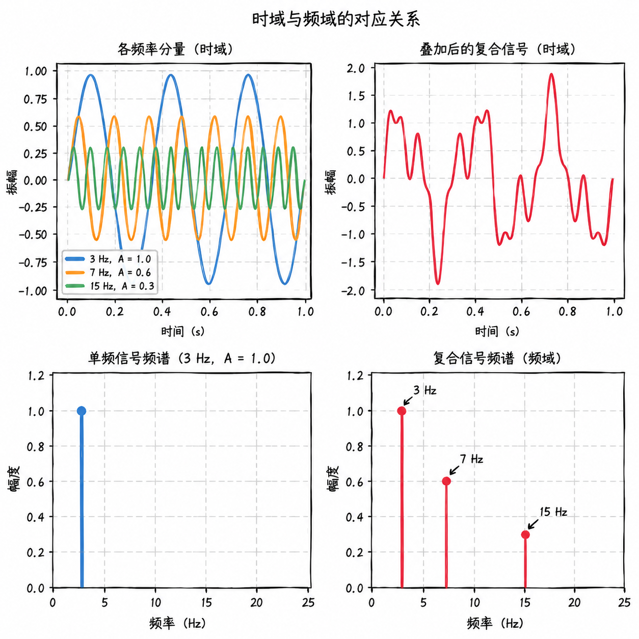
First look at the top row. The upper left shows the time-domain waveforms of three components, each with a different color and rhythm—at this stage they're still distinguishable. The upper right is the composite signal after adding them together, chaotic and disordered.

Now look at the bottom row. The lower left is the frequency domain of a single 3 Hz sine wave: energy is mainly concentrated around 3 Hz, with height corresponding to amplitude 1.0. When FFT processes finite-length data in practice, there may be some spread around the main frequency, but the most prominent peak remains near 3 Hz.

The lower right is the frequency domain of the composite signal: three vertical lines stand at 3, 7, and 15 Hz, with heights of exactly 1.0, 0.6, and 0.3. That chaotic waveform in the time domain reveals its structure in the frequency domain.

Fourier Transform and FFT

The tool used to compute the frequency spectrum from the time-domain waveform is called theFourier Transform(Fourier Transform). Conversely, restoring the time-domain waveform from the spectrum is called the inverse Fourier transform.

The Fourier transform is somewhat like a prism separating light: white light appears as one color, but when separated you can see different color components; a waveform appears chaotic, but after transformation you can see different frequency components.

In actual computation, a discrete version is used, calledFast Fourier Transform(FFT, Fast Fourier Transform). FFT outputs a set of complex number results, each result corresponding to a frequency bin. When plotting a spectrum, the magnitude of these results is typically taken to represent the intensity of the corresponding frequency component.

FFT itself only gives bin indices like "0th, 1st, 2nd..." To convert the indices to actual frequencies, you need to know the sampling rate and the number of points.

Assume the sampling rate is $f_s$ and the FFT size is $N$. Without additional zero-padding, the observation time corresponding to $N$ samples is:

T_{\text{obs}} = \frac{N}{f_s}

For example, if the sampling rate is 1000 Hz and 1000 points are taken, the observation time is 1 second. The longer the observation time, the finer the frequency bins; the frequency spacing between adjacent bins is:

\Delta f = \frac{f_s}{N}

In this example, $\Delta f = 1000/1000 = 1$ Hz. The frequency corresponding to the $k$-th bin is $k \cdot \Delta f$. The horizontal axis of the FFT plot needs to be interpreted from the sampling rate and number of points.

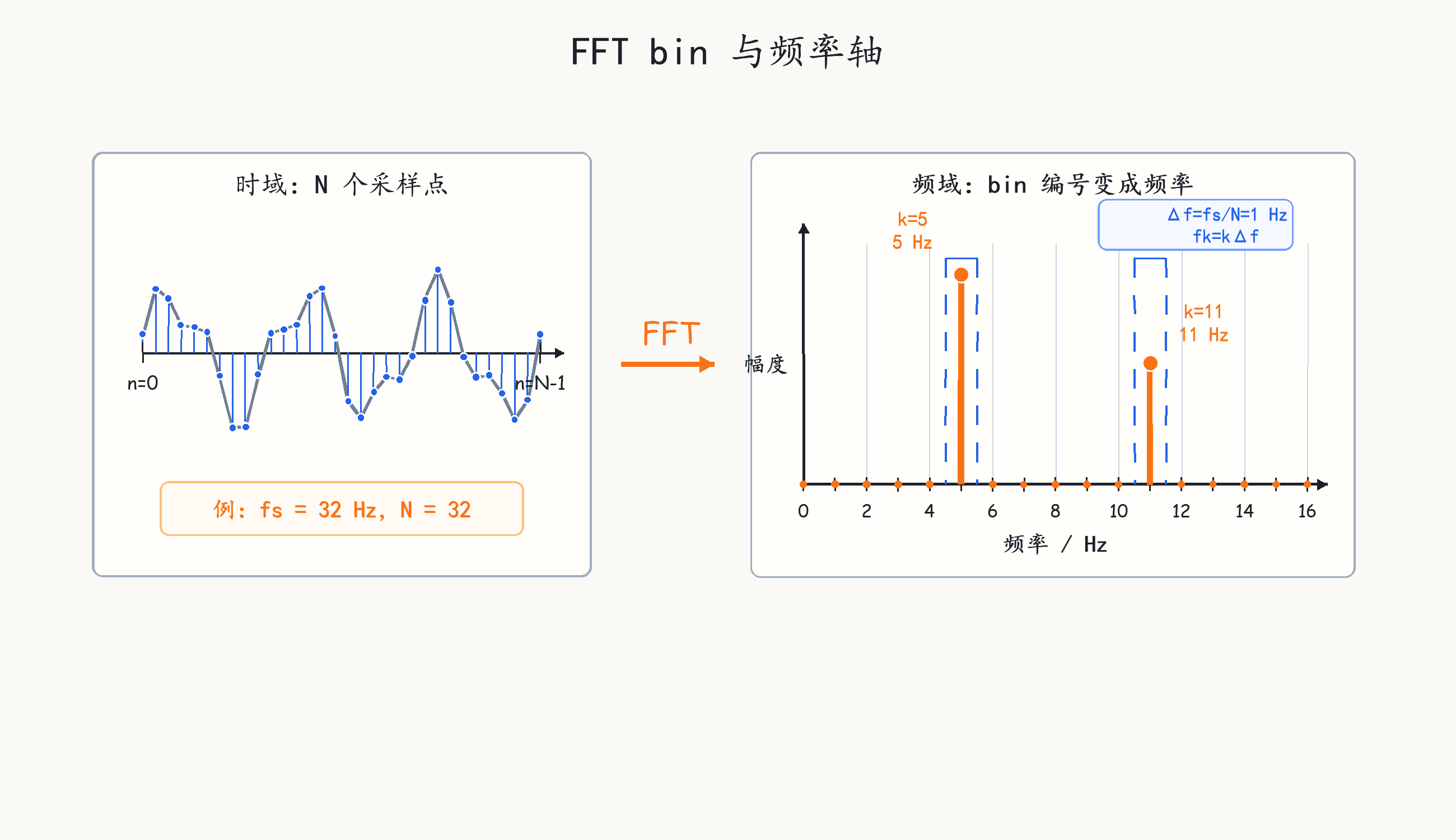
Figure 2.5 shows the correspondence between time-domain samples and frequency-domain bins together. On the left is a sequence of sample points, on the right are the FFT frequency bins. Once the sampling rate and number of points are determined, the frequency axis can be labeled according to $\Delta f=f_s/N$.

Frequency Resolution

The $\Delta f$ mentioned earlier is the spacing of frequency bins. When reading a spectrum, another more practical question arises: can two real spectral lines that are very close together be distinguished? This capability is usually calledFrequency Resolution, primarily determined by the observation time $T_{\text{obs}}$:

\Delta f_{\text{res}} \approx \frac{1}{T_{\text{obs}}}

Observing for 1 second allows resolving differences of about 1 Hz; observing for 0.1 second only allows resolving differences of about 10 Hz. The longer the observation time, the smaller the frequency separation that can be resolved.

Zero-padding can make the FFT output more points, reduce the bin spacing, and make the spectrum plot look finer; but it cannot separate two real frequency components that are inherently inseparable. True frequency resolution capability is primarily determined by observation time.

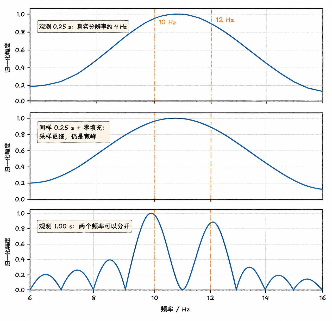
Figure 2.6 Observation time, zero-padding, and frequency resolution

In Figure 2.6, the first two rows have the same observation time, and zero-padding only makes the spectral curve finer; in the third row, after the observation time increases, the two closely spaced frequency peaks separate.

The time domain shows voltage changing with time, the frequency domain shows frequency components; FFT is a common tool for transforming sampled data into the frequency domain.

2.3 Sampling Theorem

The sinusoids, superposition, and spectra discussed earlier were all described in a "continuous-time" framework: the signal has a value at every instant. But computers cannot process continuous signals. Computers can only store numbers, one at a time, not infinitely many.

To make computers process signals, continuous signals must be converted into a sequence of discrete values—this process is calledsampling。

Sampling Rate and Nyquist Frequency

Sampling means taking a point at fixed time intervals, recording the signal value at that moment, and discarding all other moments. The question is: with so much information discarded, can the original signal still be recovered?

How many points are taken per second is thesampling rate $f_s$, in Hz. The higher the sampling rate, the more accurate the reconstruction, but storage and transmission have costs. So what is the minimum required?

Assume the signal's highest frequency is 10 Hz, meaning it completes at most 10 full oscillations per second. To capture this oscillation, sampling must occur at least twice per cycle; the sample points don't necessarily land exactly on peaks or troughs, but the sampling rate must be high enough. So the sampling rate must be at least 20 Hz.

The sampling theorem (also called the Nyquist-Shannon theorem) expresses this requirement as:

f_s > 2 f_{\max}

$f_{\max}$ is the highest frequency component contained in the signal. Under ideal band-limited conditions, as long as the sampling rate is strictly greater than twice the maximum frequency, the signal can be completely reconstructed. Real systems must also account for noise, filter roll-off, and sampling clock errors, so engineering practice typically includes a margin.

This boundary at $f_s / 2$ has a specific name, called theNyquist frequency. A sampling rate of 1000 Hz corresponds to a Nyquist frequency of 500 Hz, meaning this sampling rate can correctly capture signal components below 500 Hz.

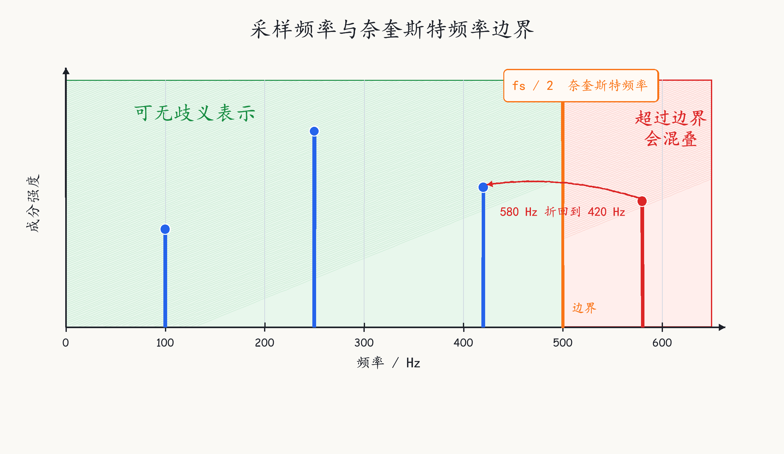
Figure 2.7 Sampling Frequency and Nyquist Frequency Boundary

Figure 2.7 illustrates this condition on the frequency axis. The green region represents the frequency range that can be unambiguously represented at the current sampling rate; components exceeding $f_s/2$ will fold back, and the frequency they exhibit after sampling is no longer the original true frequency.

Sampling and Aliasing

Figure 2.8 shows an experiment with three different sampling rates applied to a 10 Hz sine wave. The gray line is the original signal, orange dots are the sampling points, and the blue dashed line is the waveform reconstructed from the sampling points.

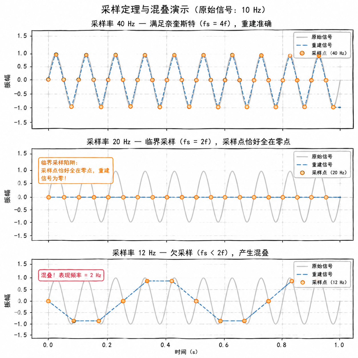
Figure 2.8 Sampling Theorem and Aliasing Demonstration

First row, 40 Hz sampling ($f_s = 4f$). Far exceeds the Nyquist criterion, the orange sampling points are sufficiently dense, and the blue reconstructed waveform nearly perfectly overlaps with the gray original signal.

Second row, 20 Hz sampling ($f_s = 2f$). Right at the critical boundary. In this example, the sampling points happen to fall exactly at the zero-crossings of the sine wave, resulting in a reconstructed zero line. This is a special case where the sampling starting point aligns precisely with the signal phase; the problem is that $f_s=2f$ has no margin, and practical systems cannot rely on this boundary condition. Therefore, the strict condition is written as $f_s>2f_{\max}$, and engineering practice adds additional margin.

Third row, 12 Hz sampling ($f_s < 2f$). The sampling rate is below the Nyquist requirement, causingaliasing: observe the blue dashed line, the reconstructed waveform is no longer 10 Hz, but has become a slowly oscillating 2 Hz low-frequency signal. The original high-frequency signal is 'disguised' as a non-existent low-frequency signal.

Why does it become 2 Hz? In this example, the signal frequency falls between $f_s/2$ and $f_s$, and the apparent frequency after aliasing can be calculated using the following folding relationship:

f_{\text{alias}} = f_s - f_{\text{signal}} = 12 - 10 = 2\,\text{Hz}

Higher frequencies undergo multiple folds, but the intuition is the same: components exceeding the Nyquist frequency are folded back into the low-frequency region.

Once aliasing occurs, it is irreversible. You cannot distinguish from the existing sampled data whether that 2 Hz is a 'real 2 Hz signal' or an 'illusion of 10 Hz aliased down.' This is why the sampling rate must satisfy the Nyquist criterion, and filters are often used before sampling to block excessively high frequency components.

ADC Sampling Data

In a radar receiver, there is a key component called ananalog-to-digital converter(ADC, Analog-to-Digital Converter), whose job is to sample the echo signal—converting continuous analog voltage into discrete digital sequences for subsequent digital signal processors.

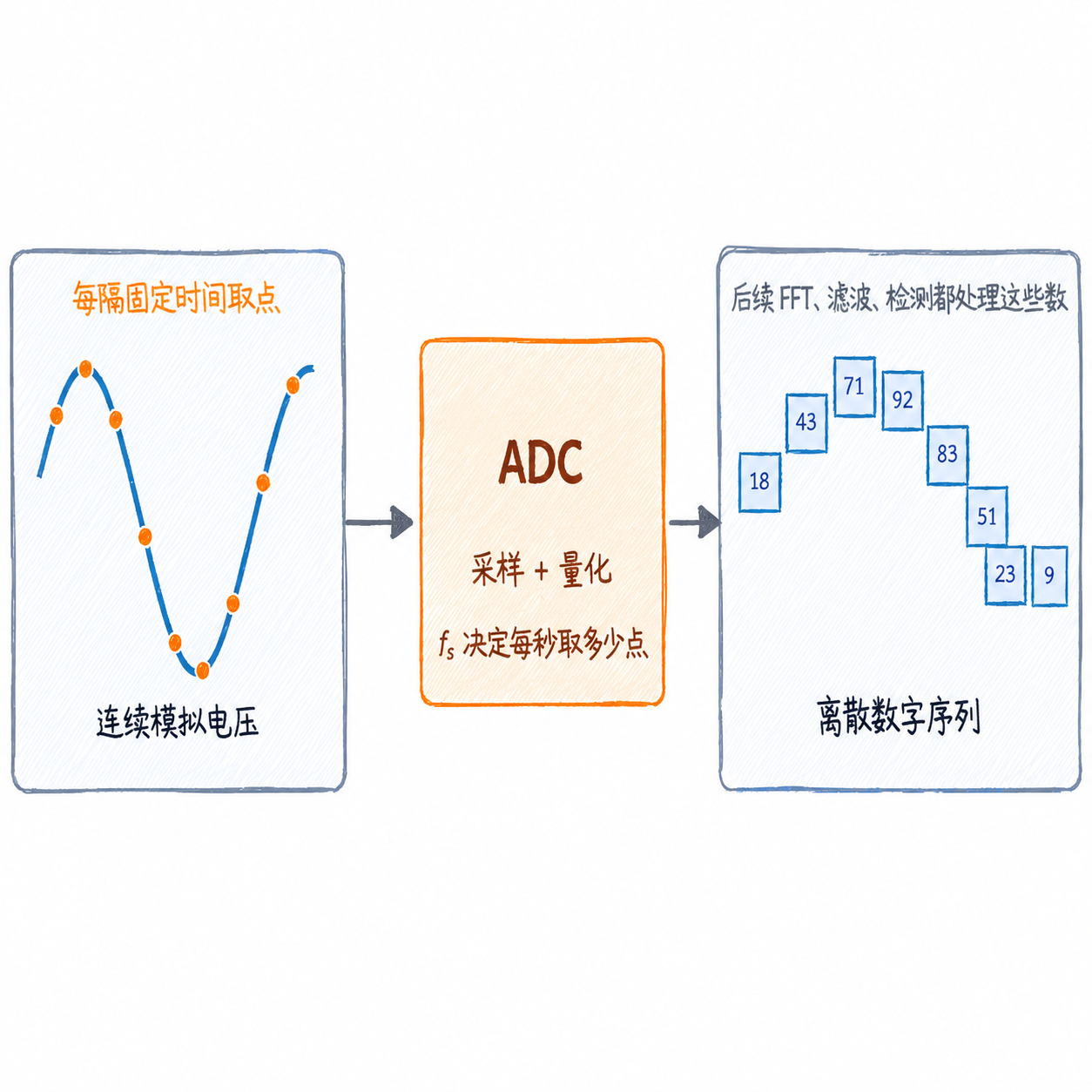
Figure 2.9 ADC converts continuous voltage into digital sequence

Figure 2.9 shows only the ADC's role in this section: on the left is continuously varying analog voltage, in the middle the ADC samples at a fixed rate and quantizes, on the right it becomes a string of numbers. The subsequent FFT, filtering, and detection all process these numbers.

The ADC sampling rate directly affects how much bandwidth the radar can process. If the equivalent bandwidth is 50 MHz, the sampling rate typically needs to be at least 100 MHz or higher, coordinated with front-end filtering and downconversion design. Higher sampling rates make ADCs more expensive and power-hungry, so engineering requires careful tradeoffs.

The sampling theorem provides a baseline: components above the Nyquist frequency will fold back into the low-frequency range, and after aliasing it becomes very difficult to distinguish their sources.

2.4 Complex Numbers, Phase, and I/Q Data

The sine waves discussed in previous sections are all real signals: amplitude can be positive or negative, but always real. In radar signal processing, we also encounter complex data.

Why do we need complex numbers? The key is phase.

Phase Information

If we write the sine wave's "starting point" into the formula as well, it becomes:

s(t) = A \sin(2\pi f t + \varphi)

The additional $\varphi$ here isphase. Phase describes the sine wave's "starting point" or "position in its cycle". Two sine waves with the same frequency and amplitude will be offset if their starting points differ.

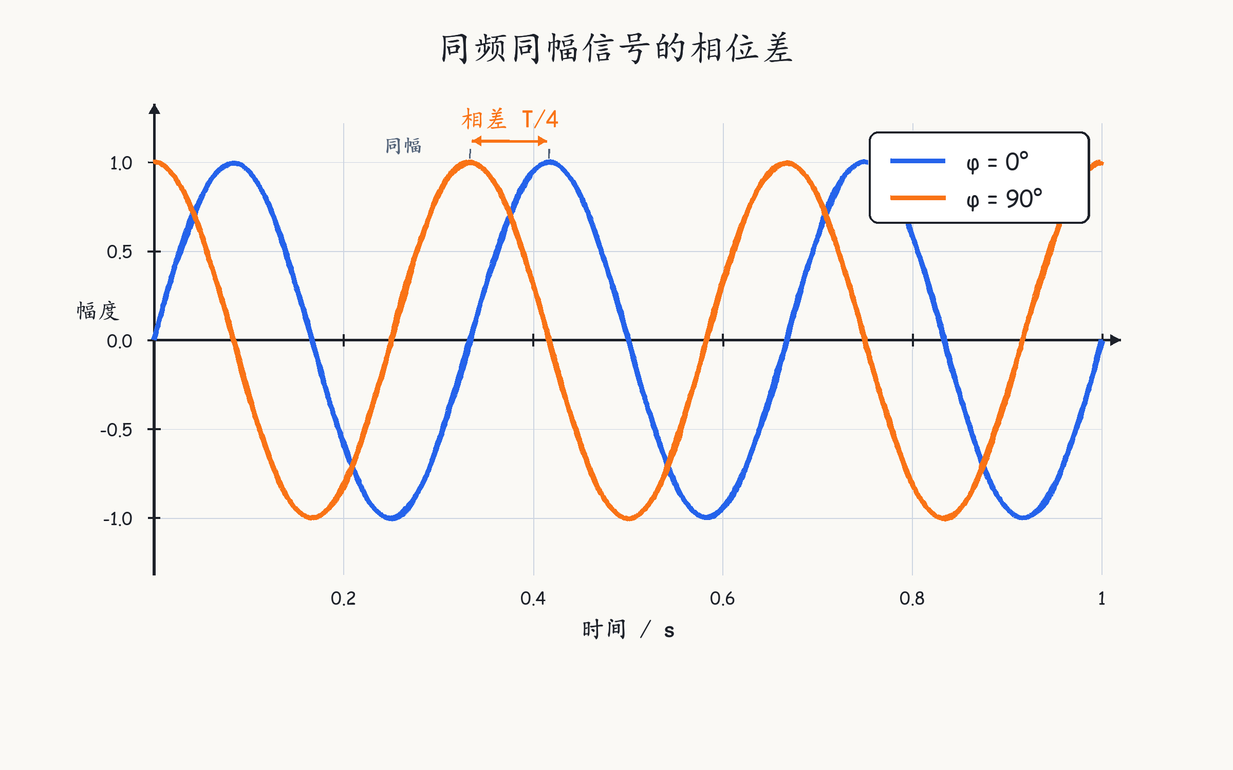
Figure 2.10 Phase difference of same-frequency, same-amplitude signals

The two curves in Figure 2.10 have identical frequency and amplitude, only their starting points are offset. Phase is used to record this offset amount.

Phase is very important in radar. When we discuss velocity measurement later, you'll see that moving targets cause the echo's phase to rotate over time, and the rotation rate corresponds to the target's velocity. If only amplitude is recorded, phase information is lost, and velocity cannot be measured.

Complex Numbers and I/Q Components

Complex numbers can simultaneously record amplitude and phase. A complex sample can be written as:

$$ s = I + jQ $$

$I$ and $Q$ are two real numbers, $j$ is the imaginary unit. $I$ is calledin-phase component(In-phase), $Q$ is calledquadrature component(Quadrature). The two real numbers together form a complex sample.

This complex number can also be plotted on a plane. The horizontal axis represents $I$, the vertical axis represents $Q$, and the sample corresponds to a point on the plane, or an arrow from the origin to that point.

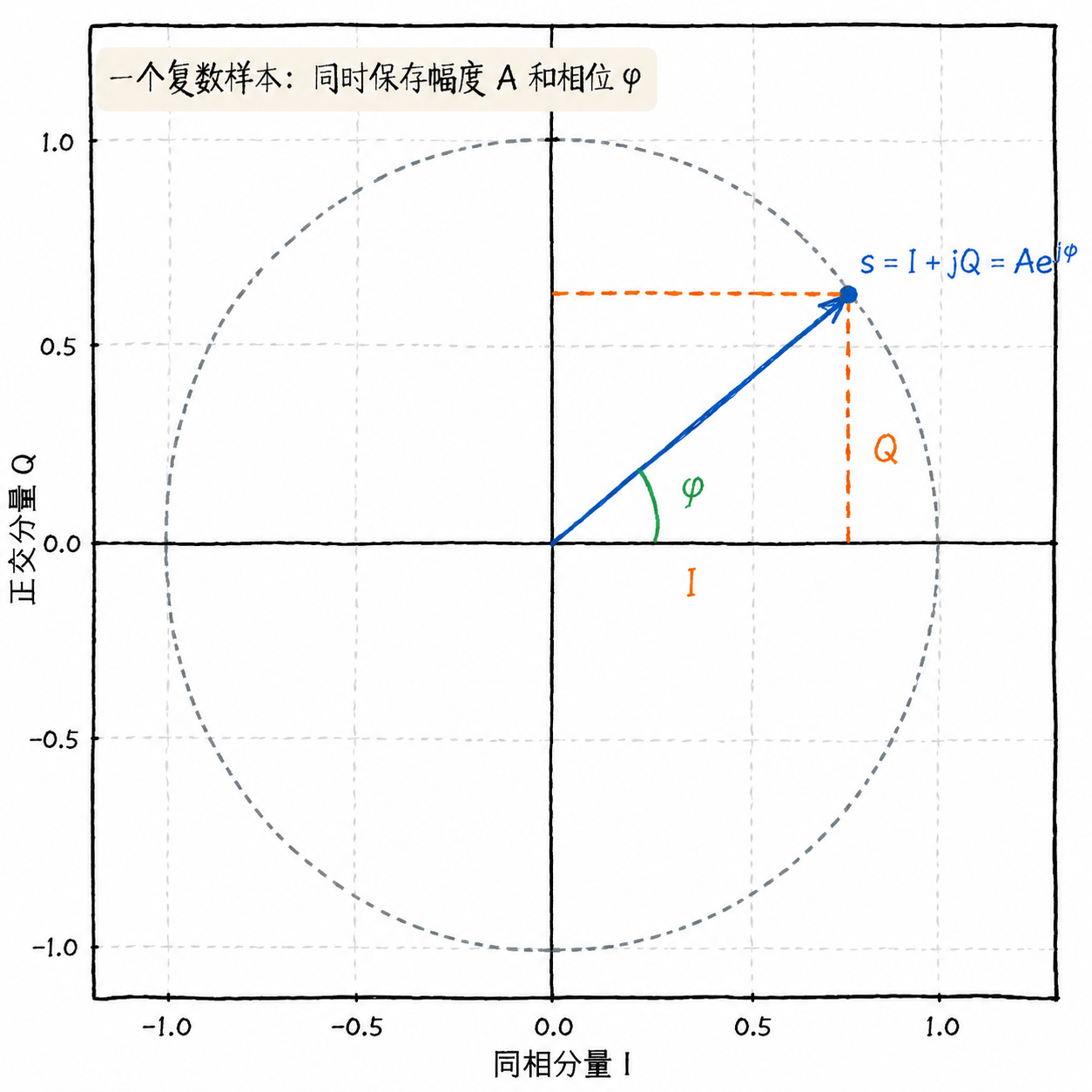
In Figure 2.11, the length of the blue arrow represents amplitude, and the angle the arrow makes with the horizontal axis represents phase. $I$ and $Q$ are two coordinates of the same complex sample and cannot be interpreted as two independent ordinary curves.

Let's look at a specific numerical example. Suppose an echo sample point has I/Q values $I=3$ and $Q=4$; the corresponding complex number is

$$ s = 3 + j4 $$

In radar data, $I=3$ and $Q=4$ describe the same echo sample point. From these two numbers, we can calculate the amplitude $A=\sqrt{3^2+4^2}=5$ and phase $\varphi=\operatorname{atan2}(4,3)\approx 53^\circ$. If only the amplitude 5 is saved, both $3+j4$ and $3-j4$ reduce to just "same intensity"; retaining I/Q allows subsequent processing to distinguish their phase directions. Velocity estimation, coherent integration, and other processing rely on precisely these phase differences.

To calculate amplitude from $I$ and $Q$, use the Pythagorean theorem:

A = \sqrt{I^2 + Q^2}

Phase is typically calculated using $\operatorname{atan2}(Q,I)$, which distinguishes between different quadrants. The same sample can also be written in polar form:

s = A e^{j\varphi}

$A$ is the amplitude and $\varphi$ is the phase. The rectangular form $I+jQ$ and polar form $Ae^{j\varphi}$ are simply two ways of writing the same complex number.

Origin of I/Q Data

Radar receivers typically output I/Q data on two channels. Thequadrature demodulationprocess can be understood by first looking at the result: the receiver uses two reference signals with a 90° phase difference to separately process the same echo, with one channel yielding $I$ and the other yielding $Q$.

This section does not expand on the circuit details of mixers and low-pass filters; it suffices to remember that I/Q comes from the receiver's demodulation and sampling chain and is used to preserve the echo's amplitude and phase.

I/Q is a very common storage format in radar data. A complex sample can simultaneously record amplitude and phase, which will be used in subsequent range processing, velocity processing, and matched filtering.

I/Q samples use two numbers to store amplitude and phase, with phase being used in velocity processing later.

2.5 Practice Problems

This section reviews several basic concepts from this chapter through exercises: frequency and period, spectrum readings, aliasing determination, frequency resolution, and the amplitude and phase of I/Q samples.

Frequency and Period

A sinusoidal signal has a period of $T = 0.02$ s. What is its frequency?

Solution: From $f = 1/T$, we obtain

f = \frac{1}{0.02} = 50\,\text{Hz}

Spectrum Reading

A signal's spectrum has two spectral lines: one at 100 Hz with height 3 V, and another at 250 Hz with height 1 V.

(a) Write the time-domain expression for this signal (ignoring phase).

(b) If this signal is to be sampled, what is the minimum required sampling rate?

Solution: Each spectral line in the frequency spectrum corresponds to a sinusoidal component, so the time-domain signal can be written as

s(t) = 3\sin(2\pi \cdot 100 \cdot t) + 1\sin(2\pi \cdot 250 \cdot t)

The highest frequency component in this signal is 250 Hz. According to the sampling theorem, the sampling rate must satisfy

f_s > 2f_{\max} = 2 \times 250 = 500\,\text{Hz}

Therefore, the sampling rate must be at least greater than 500 Hz.

Aliasing Detection

You sample a signal at 800 Hz. The signal contains three frequency components: 100 Hz, 300 Hz, and 500 Hz. Which components will experience aliasing? What frequencies will they appear as after aliasing?

Solution: The Nyquist frequency corresponding to an 800 Hz sampling rate is

\frac{f_s}{2} = 400\,\text{Hz}

Therefore, both 100 Hz and 300 Hz are below 400 Hz and will not alias; 500 Hz is above 400 Hz and will alias. The apparent frequency after aliasing is

f_{\text{alias}} = f_s - f_{\text{signal}} = 800 - 500 = 300\,\text{Hz}

In other words, the 500 Hz component will fold back to 300 Hz and coincide with the existing 300 Hz component.

Frequency Resolution

A radar continuously observes a target for 0.05 seconds. The target echo may contain two Doppler frequency components: 1000 Hz and 1015 Hz. Can these two components be separated in the frequency spectrum? If not, what is the minimum observation time required?

Solution: The frequency resolution is approximately

\Delta f = \frac{1}{T_{\text{obs}}}

Substituting the observation time $T_{\text{obs}} = 0.05$ s, we get

\Delta f = \frac{1}{0.05} = 20\,\text{Hz}

The two frequency components differ by only 15 Hz, which is less than 20 Hz, so they cannot be separated with the current observation time.

To resolve a 15 Hz difference, we need to satisfy

T_{\text{obs}} \ge \frac{1}{15} \approx 0.067\,\text{s}

This means an observation time of at least approximately 67 ms is required.

I/Q Amplitude and Phase

A complex sample point is $s = 3 + j4$. What is its magnitude? What is its phase approximately?

Solution: The magnitude is

A = \sqrt{I^2 + Q^2} = \sqrt{3^2 + 4^2} = 5

The phase is

\varphi = \operatorname{atan2}(4,3) \approx 53.1^\circ \approx 0.93\,\text{rad}

This sample can be understood as an arrow in the I/Q plane with length 5, rotated approximately $53.1^\circ$ from the I axis.