Chapter 4: Range Measurement
4.1 Time Delay to Range
The receiver records the echo from a single transmitted pulse as a sequence of samples; when multiple pulses are transmitted consecutively, these echoes can be arranged into a matrix. Range processing first examines only one fast-time record: looking along the samples within a single pulse, the later an echo peak appears, the farther the target typically is.
Imagine the receiver records an echo waveform. The horizontal axis represents sample points, and the vertical axis represents echo amplitude. When a peak appears at some position, the first engineering question to answer is: how many meters does this peak correspond to?
Delay-Range Formula
Standing in a valley and shouting, you hear an echo after a while. If you know the speed of sound propagation, you can calculate the distance to the valley wall. Radar ranging follows the same principle, except it replaces sound waves with electromagnetic waves and human ears with receivers.
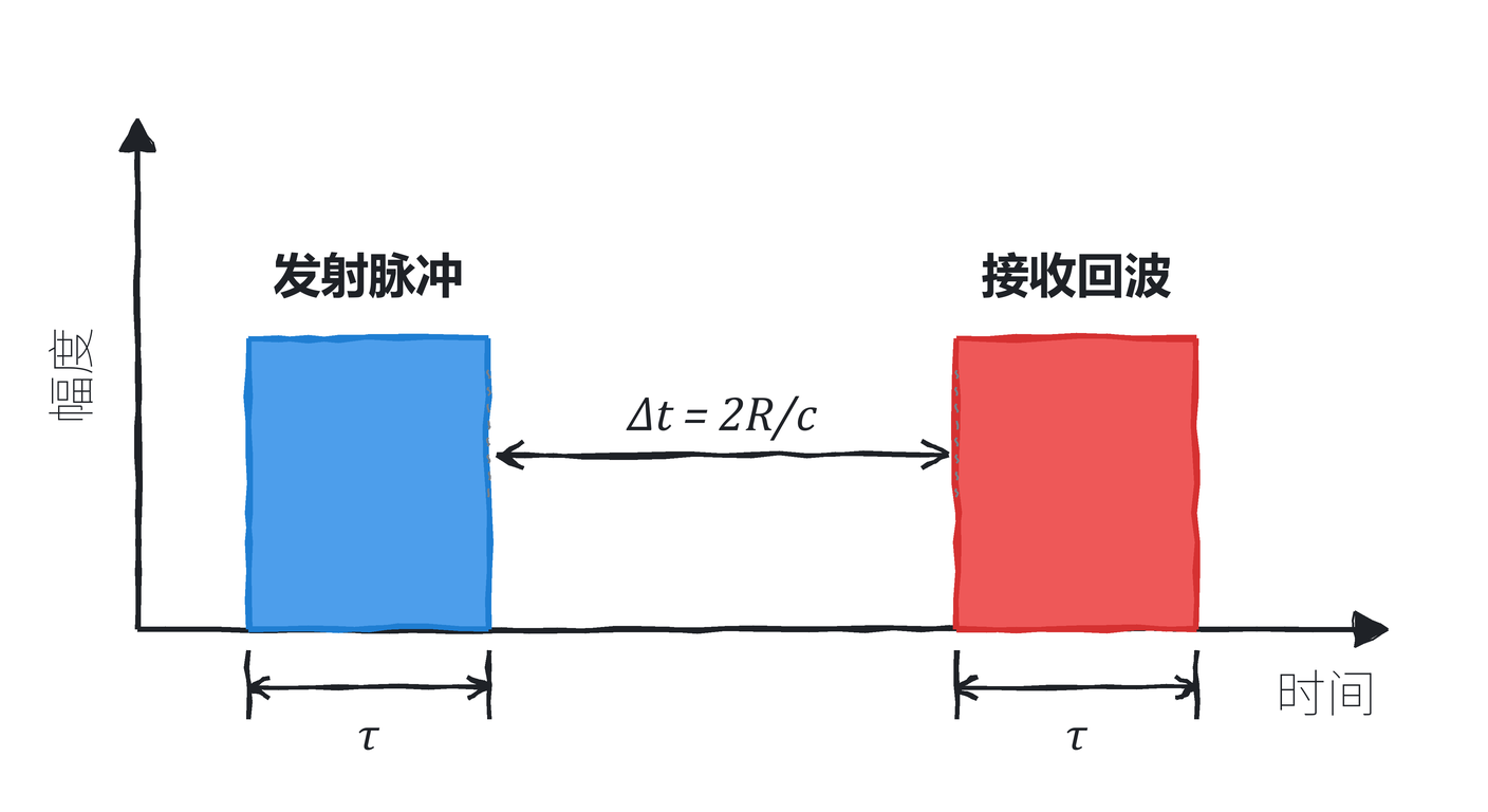
Electromagnetic waves propagate at the speed of light $c \approx 3\times10^8\,m/s$. When the target distance is $R$, the electromagnetic wave travels first from the radar to the target, then reflects back from the target to the radar, for a total path of $2R$. If the echo arrives $\Delta t$ later than the transmitted signal, then
Rewriting yields the range equation:
The factor of $2$ in the denominator comes from the round-trip path. The radar measures the total time from transmission to reception, not the one-way time.
For example, if the echo delay is $6.67\,\mu s$, the target range is approximately
Conversely, if the target range is $150\,km$, the round-trip time difference is
The first layer of meaning in the ranging problem is the time measurement problem. How late the echo returns determines roughly how far away the target is.
Here we need to distinguish between two terms. The range equation tells us at what distance a single echo peak is located; range resolution tells us whether two nearby targets can be separated. The position estimate of a single target can be very fine, but if two targets have severely overlapping echoes, they may still appear as only one peak on the range-ordered echo plot.
Sample Points to Range Axis
A real receiver converts the echo into a series of samples at sampling rate $f_s$, rather than continuously recording values at all times. The time interval between adjacent samples is
Converting this time interval to a distance axis interval gives
If the sampling rate is $100\,MHz$, the distance interval corresponding to adjacent samples is
This means the distance axis can be marked at intervals of $1.5\,m$ per sample. If an echo peak arrives667 samples later than the transmit time, the corresponding time is approximately
Converting to distance gives approximately $1\,km$. In actual code, offsets such as the receive window start and filter group delay must also be subtracted, but the physical relationship remains the same: samples are first converted to time, then time is converted to distance.
$\Delta R_{\text{sample}}$ is only the distance scale corresponding to adjacent samples. Increasing the sampling rate makes the distance axis more finely marked; whether two targets can be separated also depends on how wide the target response is after receive processing. This width is determined jointly by the transmit waveform and receive processing.
4.2 Range Resolution and Pulse Width
When Can Two Targets Be Resolved
With a single target, once the echo peak is found, the distance conversion is straightforward. The complication arises when two targets are very close together. They each have an echo, and if the two echoes are separated in time, two peaks will be visible on the range-ordered output; if they overlap, the receiver may only see a wider response blob.
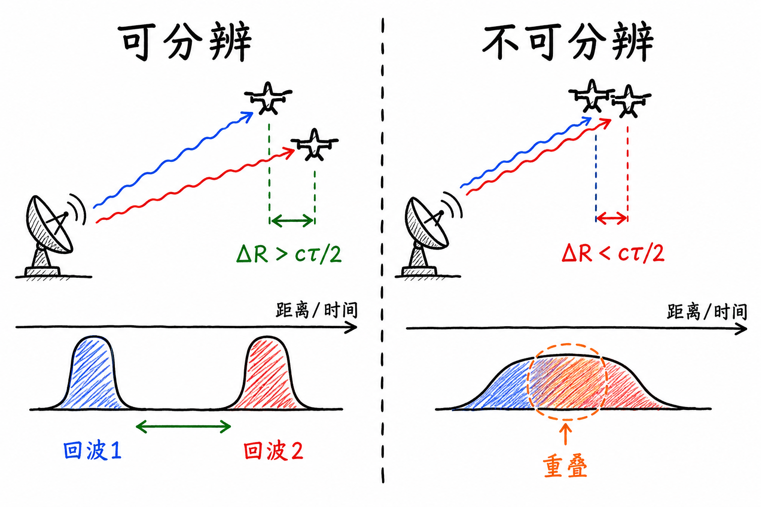
In Figure 4.2 on the left, two targets are farther apart, and the two echoes are separated in time. On the right, two targets are too close together, and the echoes overlap. In this case, even if there are many samples on the distance axis, the two targets may not be separable.
Resolution of Standard Pulses
Consider first the most common single-frequency rectangular pulse. Such a pulse has no additional internal structure, and the receiver primarily judges distance based on the arrival time of the entire echo blob. Let the transmit pulse width be $\tau$; this pulse occupies $\tau$ seconds in time, corresponds to $c\tau$ in round-trip spatial distance, which converts to one-way target distance as
This gives the order of magnitude for range resolution of an ordinary pulse radar. The shorter the pulse, the narrower the echo in time, and the easier it is to separate two nearby targets.
For example, if $\tau=1\,\mu s$, then
This means two targets within 150 m will likely merge into a single response in range. To resolve target separations of 15 m, the ordinary short pulse width would need to be reduced to approximately $0.1\,\mu s$.
Energy-Resolution Trade-off
Short pulses favor resolution but compromise energy. The shorter the pulse, the less total energy transmitted, and the weaker the echo from distant targets. Long pulses deliver more energy with better range coverage, but the echo stretches longer, degrading range resolution.
Long-range detection requires long pulses; precise ranging requires short pulses. Pulse compression resolves this contradiction: transmit with long pulses to preserve energy, then compress the return into a narrow peak to achieve resolution capability close to that of short pulses.
4.3 Pulse Compression and LFM Signals
Bandwidth and Range Resolution
Start with an ordinary single-frequency long pulse. Such a pulse has little internal structure; the main information available to the receiver is "where this energy blob begins and where it ends." When echoes from two targets are close together, the two blobs overlap substantially and still look like one stretched energy blob, making it difficult for the receiver to determine whether there is one target or two.
Pulse compression takes a different approach: still transmit with long pulses to preserve energy, but deliberately introduce identifiable variation inside the pulse—for example, frequency sweeping over time, or phase changing according to a specific pattern. This way, the receiver not only observes "roughly when this echo blob returns," but also compares: at which delay position does the internal variation pattern of the echo best align with the transmitted signal?
Thus, whether the receiver can resolve very small time misalignments depends on how rapidly and richly the pulse varies internally. The faster the variation, the wider the frequency components spread; the quantity used to characterize this range is the waveform bandwidth $B$.
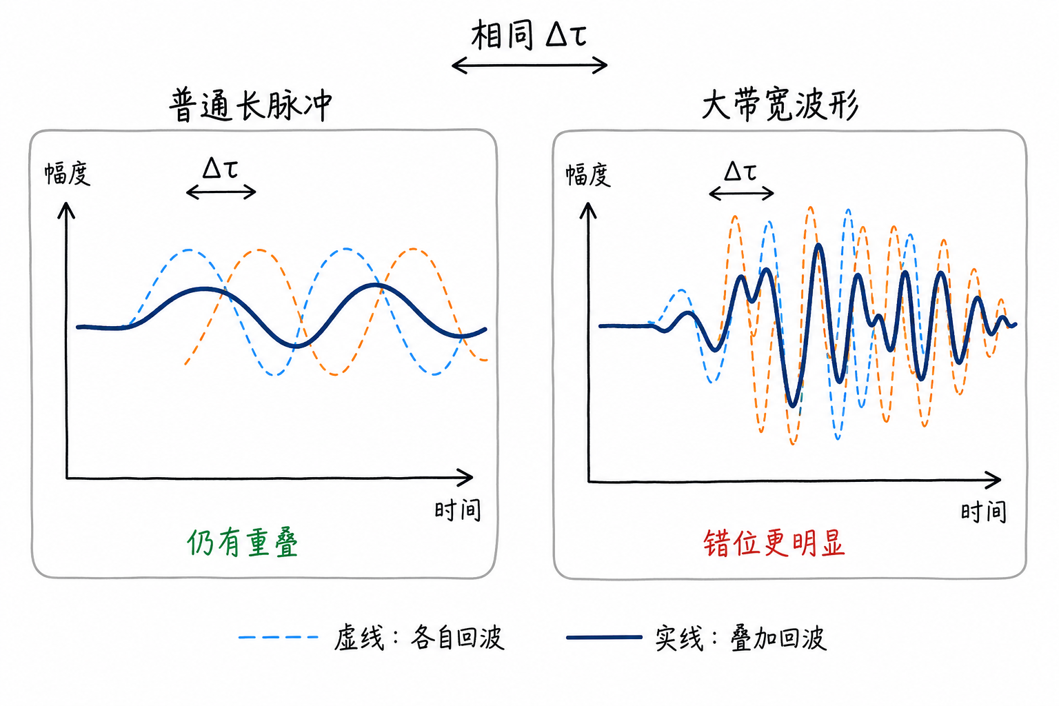
Figure 4.3 illustrates this difference. On the left, the ordinary long pulse still has substantial overlap after slight misalignment, with small waveform difference; on the right, the wide-bandwidth waveform has richer internal variation—the same misalignment causes structural misalignment, and correlation output drops more rapidly. Greater bandwidth generally indicates richer exploitable variation inside the waveform, making the system more sensitive to small time-delay differences.
This relationship can be understood at the order-of-magnitude level: after matched filtering, the temporal width of the compressed mainlobe for a wide-bandwidth pulse compression waveform decreases as bandwidth increases, commonly written as
If we estimate based on the scale of the compressed mainlobe, it can be further approximated as
Range is fundamentally derived from propagation time, so converting this temporal width to a range scale simply requires connecting back to the ranging relationship established earlier:
This formula should be distinguished from the resolution formula for ordinary pulses:
| Case | Range Resolution Formula | Primarily Influenced By |
|---|---|---|
| Ordinary single-frequency rectangular pulse | $\Delta R = c\tau/2$ | Pulse width $\tau$ |
| Wide-bandwidth pulse compression waveform | $\Delta R \approx c/(2B)$ | Waveform bandwidth $B$ |
The $c/(2B)$ here is a common engineering approximation reflecting the scale of the compressed mainlobe. Different waveforms, windowing methods, and mismatch conditions will alter mainlobe shape and sidelobe height; the key distinction here is: pulse compression shifts the resolution problem from "how short must the pulse be" to "how large is the bandwidth."
After the preceding comparison, long pulse and wide bandwidth are no longer separate matters. Long pulse provides transmission time and energy; wide bandwidth provides internal variation and the narrow mainlobe after compression. Multiplying the two together yields the time-bandwidth product:
It indicates how long a pulse lasts and how wide the frequency variation range is packed inside. A large $\tau$ means long transmission time and sufficient energy; a large $B$ means rich internal structure and a narrow mainlobe after compression.
For example, if the pulse width is $100\,\mu s$ and the bandwidth is $10\,MHz$, then
the time mainlobe width after compression is approximately
Converting to range resolution:
The transmitter still uses a $100\,\mu s$ long pulse, but the receiver achieves a range resolution of about $15\,m$.
Linear Frequency Modulation Signal
One of the most common pulse compression waveforms in engineering is theLinear Frequency Modulation Signal(Linear Frequency Modulated signal, LFM), also commonly called chirp. Its instantaneous frequency rises or falls linearly with time.
Let's first look at a slow example. Suppose there is a signal with 1 Hz in the 1st second, 2 Hz in the 2nd second, 3 Hz in the 3rd second, up to 5 Hz in the 5th second. The frequency changes, but the change is stepwise.
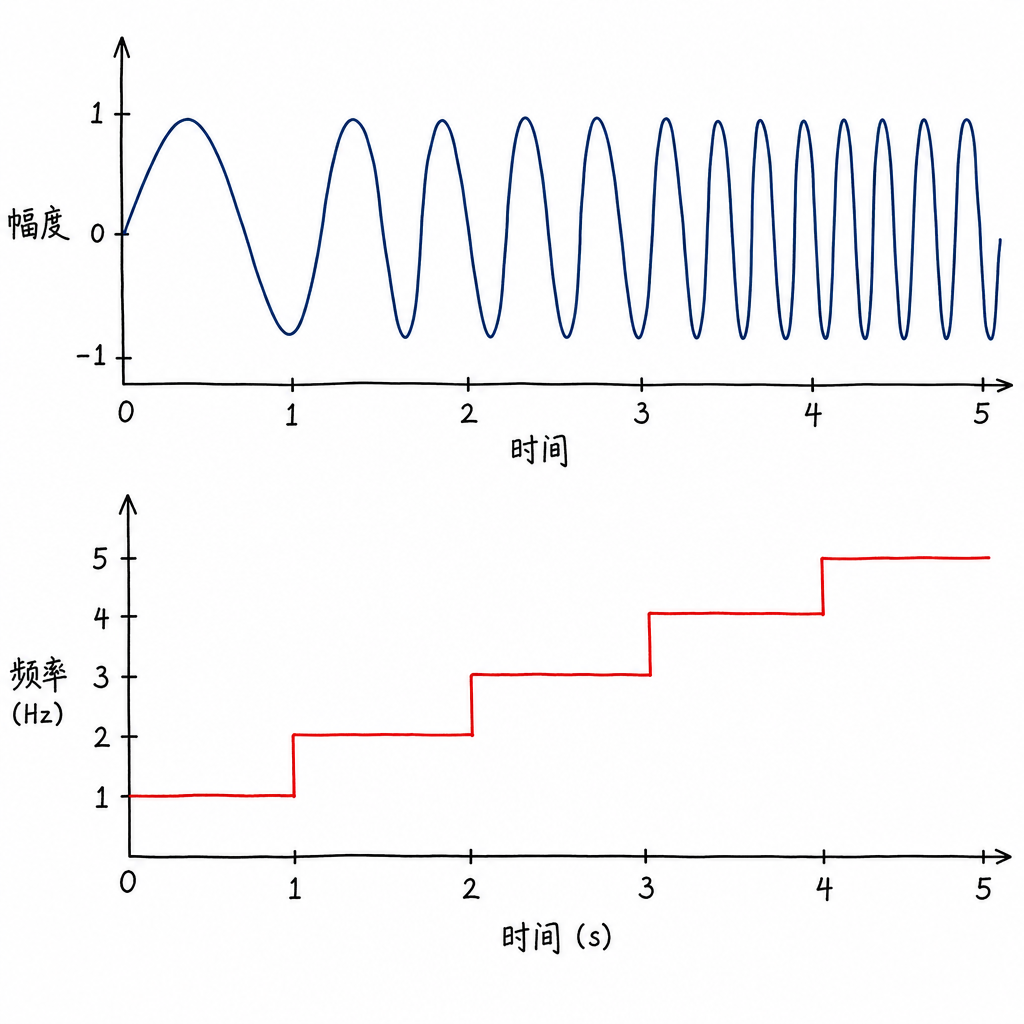
Now change the stepwise variation to continuous variation: the frequency starts at 1 Hz and smoothly rises to 5 Hz over 4 seconds. The waveform gradually becomes denser, and the frequency-time plot is a straight line with a slope.
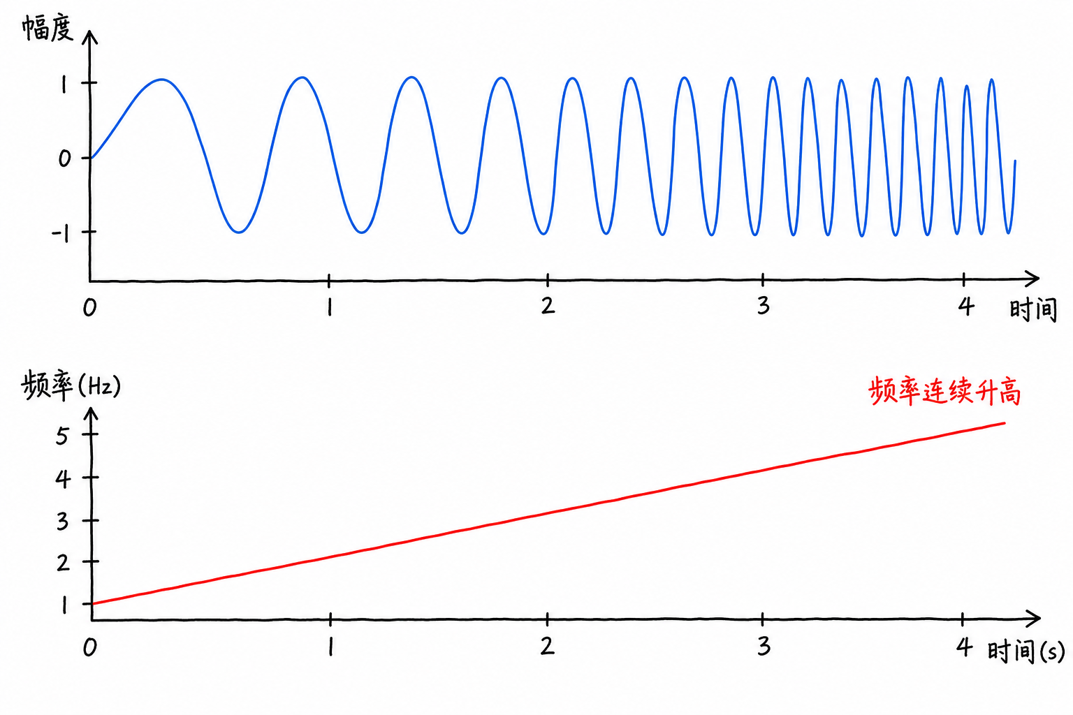
The characteristic of linear frequency modulation lies here: the frequency varies along an approximately straight line. If converted to sound, it would sound like a frequency sweep with limited duration and continuously rising pitch. Each small time segment of the LFM carries a frequency characteristic slightly different from the preceding and following segments.
Now generalize this slow example to the notation used in radar. The starting frequency is not necessarily 1 Hz, and the rate of frequency change is not necessarily 1 Hz per second. Let the instantaneous frequency be
where $f_0$ is the starting frequency and $\mu$ is the frequency modulation rate with units of Hz/s. $\mu>0$ indicates rising frequency, and $\mu<0$ indicates falling frequency.
The phase is obtained by integrating the instantaneous frequency. If the phase is denoted as $\phi(t)$, then
Therefore, the complex exponential form of the LFM can be written as
If this signal is transmitted only within a pulse of length $\tau$, it can be written as
Here $\operatorname{rect}(t/\tau)$ simply restricts the signal to within the pulse width $\tau$. If this LFM pulse sweeps a total bandwidth $B$ over time $\tau$, it means sweeping the frequency from the starting point to the endpoint, with a total range of $B$. Writing out "total change = rate of change × duration" gives
Therefore
This expression simply says: over a duration of $\tau$, the frequency sweeps a total of $B$. The larger $B$ is, the greater the frequency variation within the LFM pulse, the richer the structure available for the receiver to exploit, and the narrower the correlation peak after matched filtering.
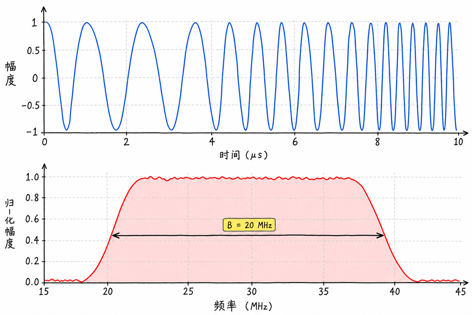
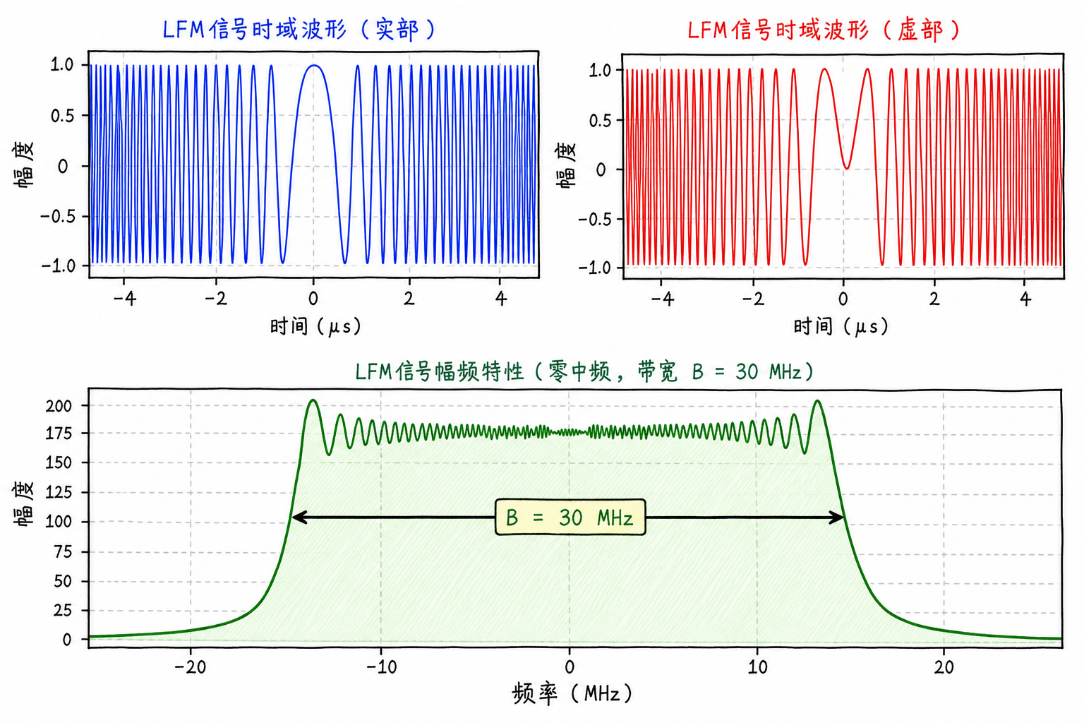
The upper part of Figure 4.6 shows the time-domain waveform, where oscillations become denser as time progresses; the lower part shows the frequency-domain energy distribution, indicating this pulse occupies a bandwidth of $B$.
Baseband Representation
Actual radar carrier frequencies are typically on the order of GHz. The receiver first performs downconversion to shift the high-frequency RF signal to a lower IF or baseband, then performs sampling and I/Q processing.
For LFM signals, after downconversion the carrier frequency term $2\pi f_0t$ can be removed, leaving the frequency modulation term:
The subscript bb stands for baseband. The baseband signal still retains the bandwidth and frequency modulation structure of the LFM, but the center frequency is shifted to near zero frequency. This processing is better suited for digital sampling and connects with the complex I/Q data from Chapter 2.
Some FMCW radars also use LFM or chirp, but those systems typically extract range through beat frequency; here we discuss LFM matched filtering in pulsed radar systems.
4.4 Matched Filtering and Range Profile
Finding Time Delay with Sliding Correlation
At this point, the transmit side already has identifiable internal structure. But the structure itself does not automatically become range peaks; the receiver must compare the echo with the known transmit signal: at which delay position do their internal variations align best?
Here's a question: how does the receiver know which signal to use for comparison with the echo?
The reference signal comes from the transmitter. The pulse transmitted by the radar is determined by the system itself: pulse width, bandwidth, chirp rate, sampling rate, and transmit time are all under the control of the transmitter and receiver. When processing echoes, the receiver can either call up the stored baseband transmit sequence or regenerate a local reference signal using these parameters. If a pulse train uses different coding or chirp parameters, the processing chain selects the corresponding reference based on the current pulse number. Matched filtering matches against this local reference, not a template guessed from the echo.
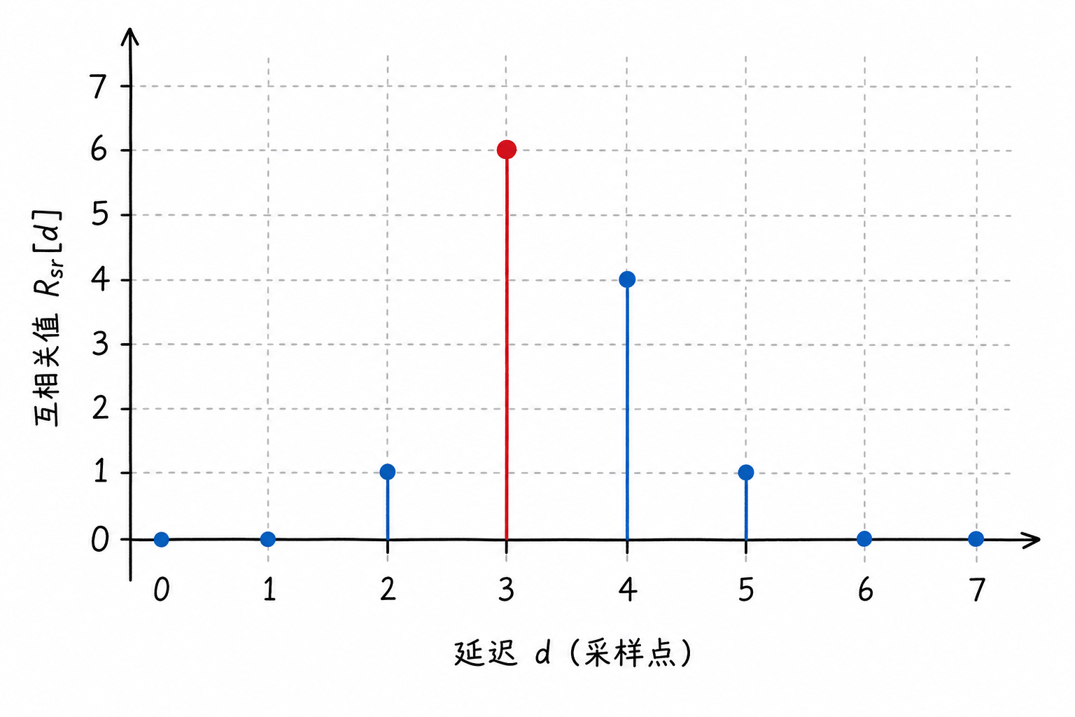
Start with a discrete example. Suppose the transmit signal has 10 sample points, with points 3 through 5 being $1,2,1$ and the rest being 0:
The echo is the same triangle shape, but delayed by 3 points overall:
Now slide the reference signal across, and for each offset $d$ perform pointwise multiplication and sum:
When the offset $d=3$, the product sum is maximum, indicating the two sequences align best at this position. The true delay is 3 sample points.
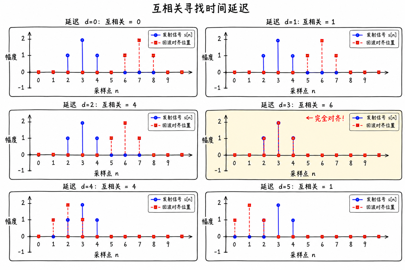
Plotting the result for each offset yields a correlation curve. The peak position corresponds to the delay.
Written as a formula, discrete cross-correlation can be expressed as
For continuous signals, replacing the sum with an integral, it can be written as
The asterisk denotes complex conjugate. Here $\tau$ is written as a positive offset: when the echo $r(t)$ arrives $\tau$ later relative to the reference signal, $r(t+\tau)$ aligns with $s(t)$. Different textbooks may adopt opposite sign conventions, but the fact that the peak position corresponds to delay remains unchanged.
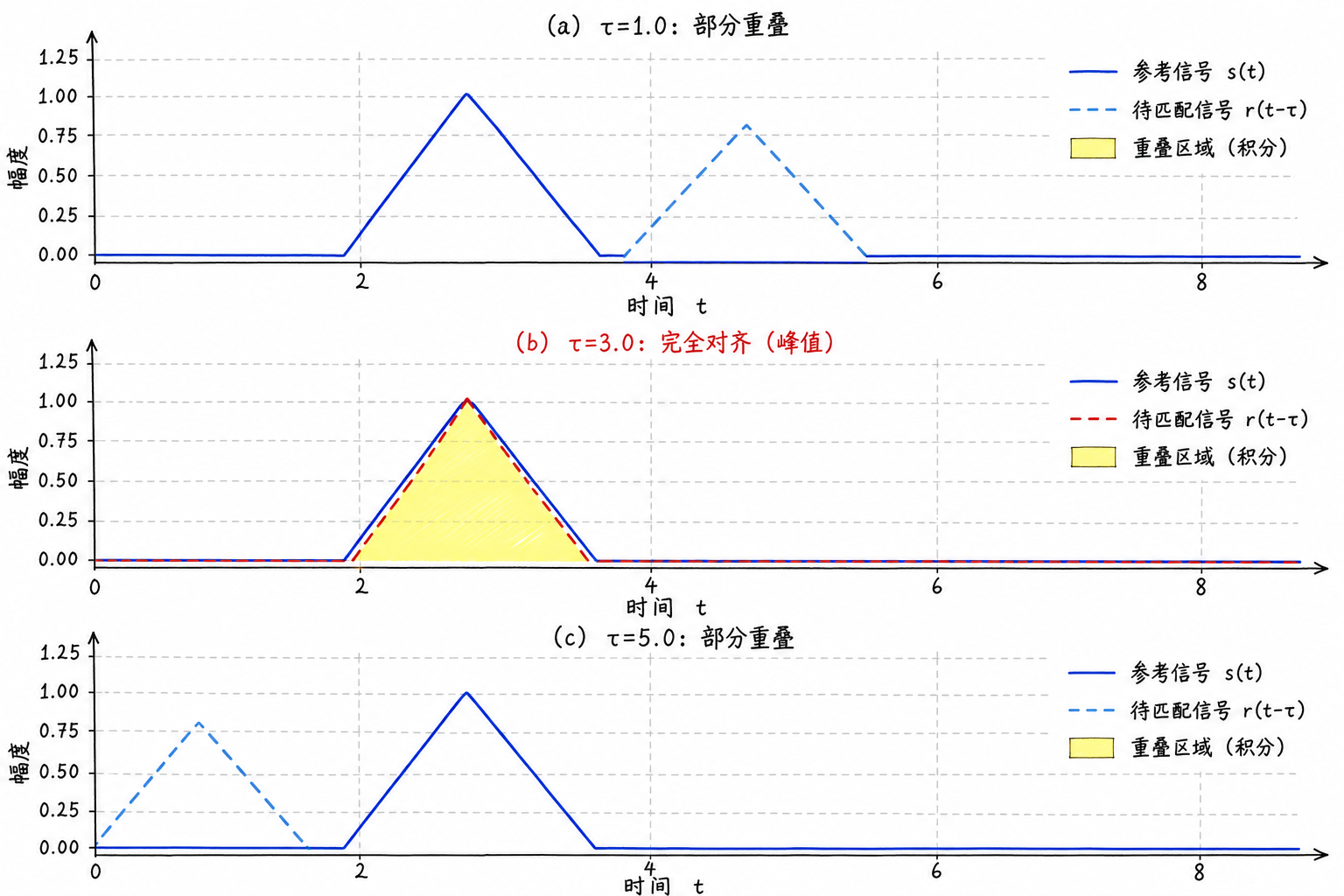
Connecting all cross-correlation values corresponding to different delays yields the cross-correlation function curve.
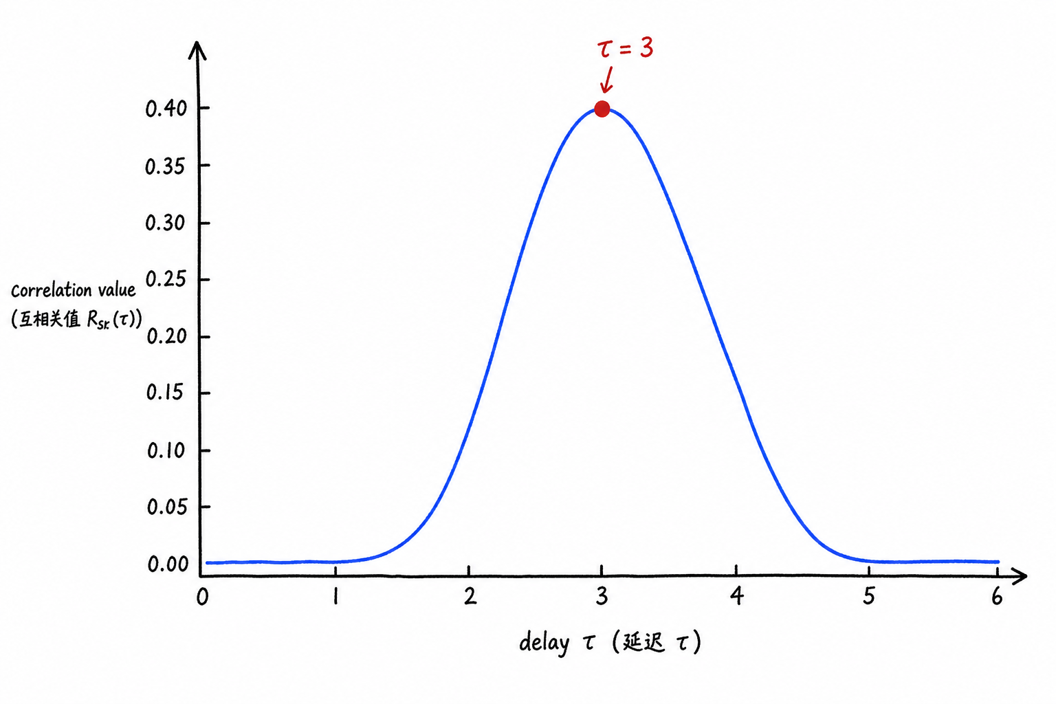
Therefore, delay estimation can be written as
The correlation peak shape varies with different waveforms. Ordinary rectangular pulses have little internal structure, so they still overlap significantly when slightly misaligned, resulting in a wide, flat correlation peak. LFM's frequency varies with time, so internal structures match simultaneously only when aligned, producing a sharper correlation peak.
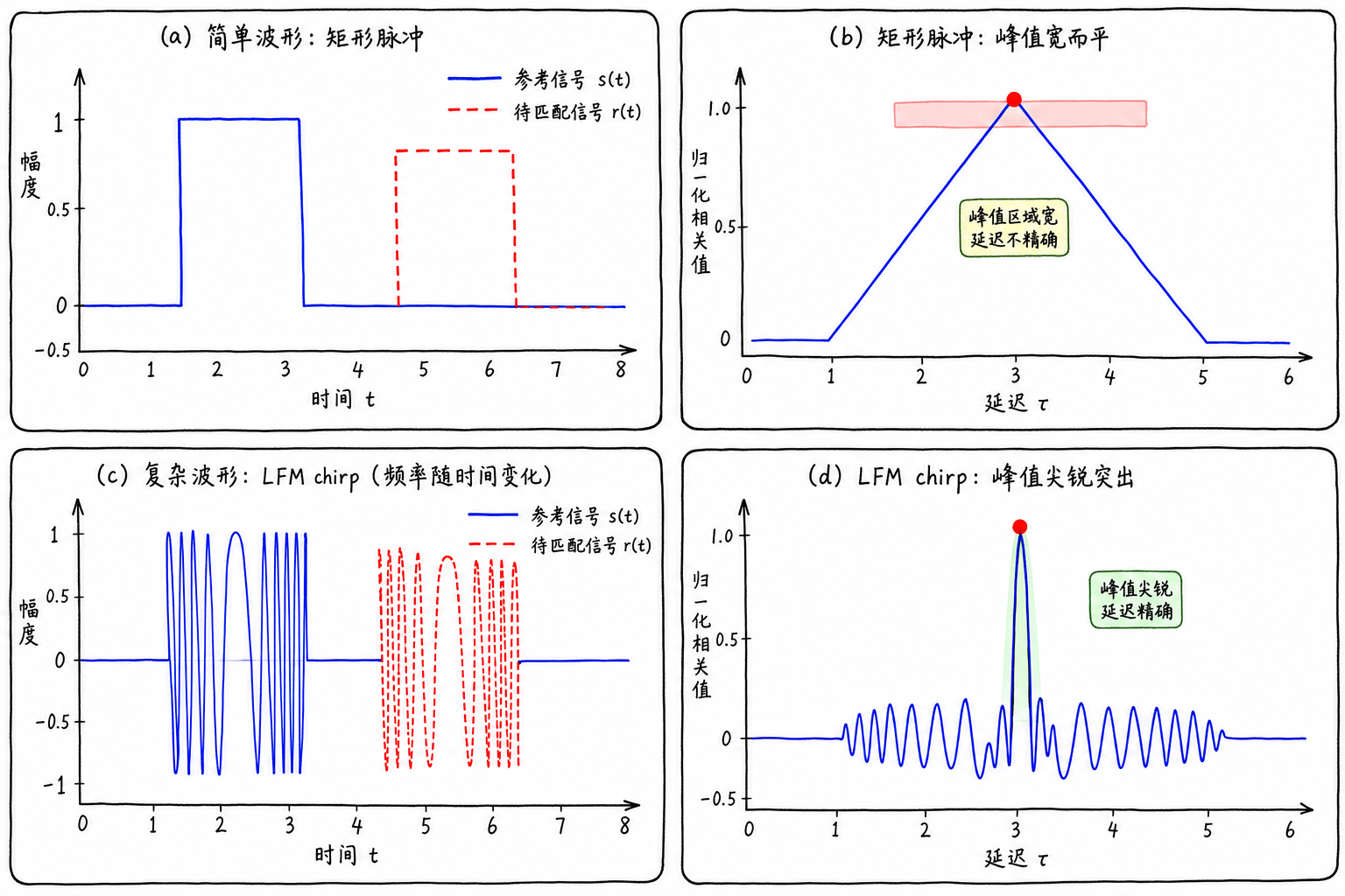
A sharper correlation peak makes the peak position easier to locate and allows two closely spaced targets to be separated more easily. This is why LFM is suitable for pulse compression.
From Cross-Correlation to Matched Filtering
Computing cross-correlation for every possible delay is computationally intensive. Radar receivers typically reformulate cross-correlation as a filter operation, passing the echo through a specialized filter whose output is the correlation result.
The impulse response of this filter is the time-reversed complex conjugate of the transmitted signal:
When the echo $r(t)$ passes through this filter, the output is
where $*$ denotes convolution. This output is equivalent to the cross-correlation result, with the peak position still corresponding to the target delay. Because the filter shape is determined by the transmitted signal, it is called amatched filter。
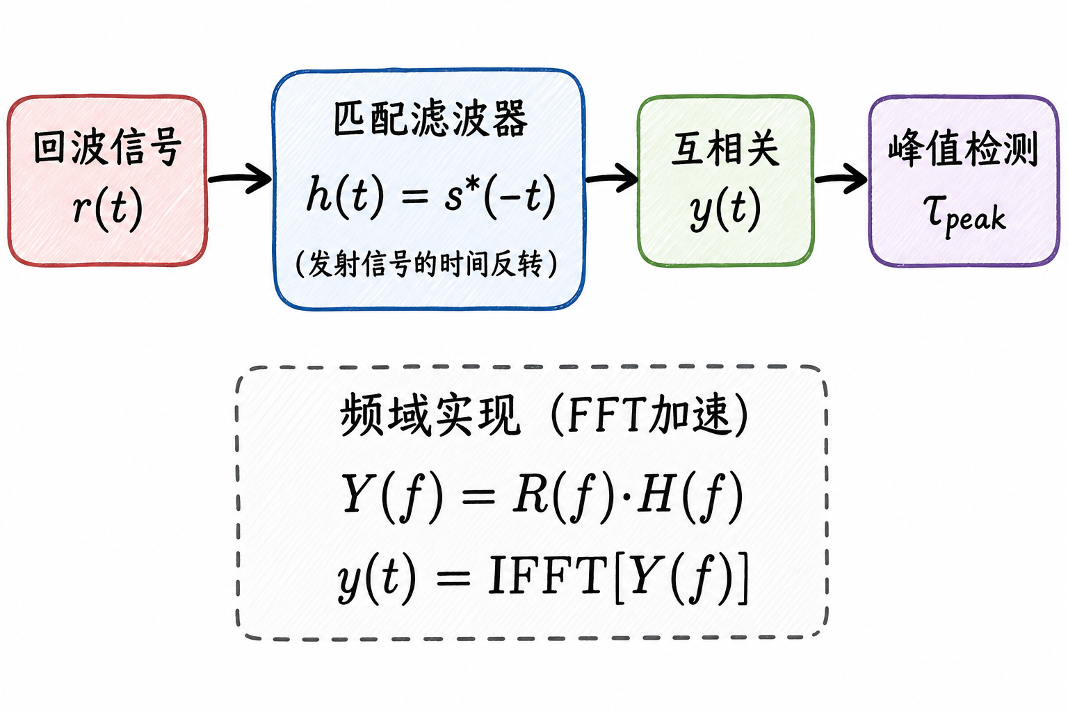
In digital radar, matched filtering is commonly implemented using FFT. According to the convolution theorem, time-domain convolution becomes frequency-domain multiplication:
Programs typically perform FFT on the echo first, multiply by the pre-computed matched filter spectrum, then perform IFFT to return to the time domain. The resulting sequence is the matched filtering output in the range dimension, also commonly called the range profile. After subtracting the receive window start time and the filter's fixed delay from the sample index where the peak occurs, the result is converted to range using the delay-to-range formula.
LFM Compression Effect, Sidelobes, and Window Functions
After matched filtering, LFM compresses a long echo into a narrow peak. Taking baseband up-chirp as an example, the transmitted signal phase contains $\pi\mu t^2$; the matched filter uses time reversal and complex conjugation, effectively adding the opposite quadratic phase. At the correct delay, these phase terms cancel each other, and energy at different time positions adds coherently, forming a high peak.
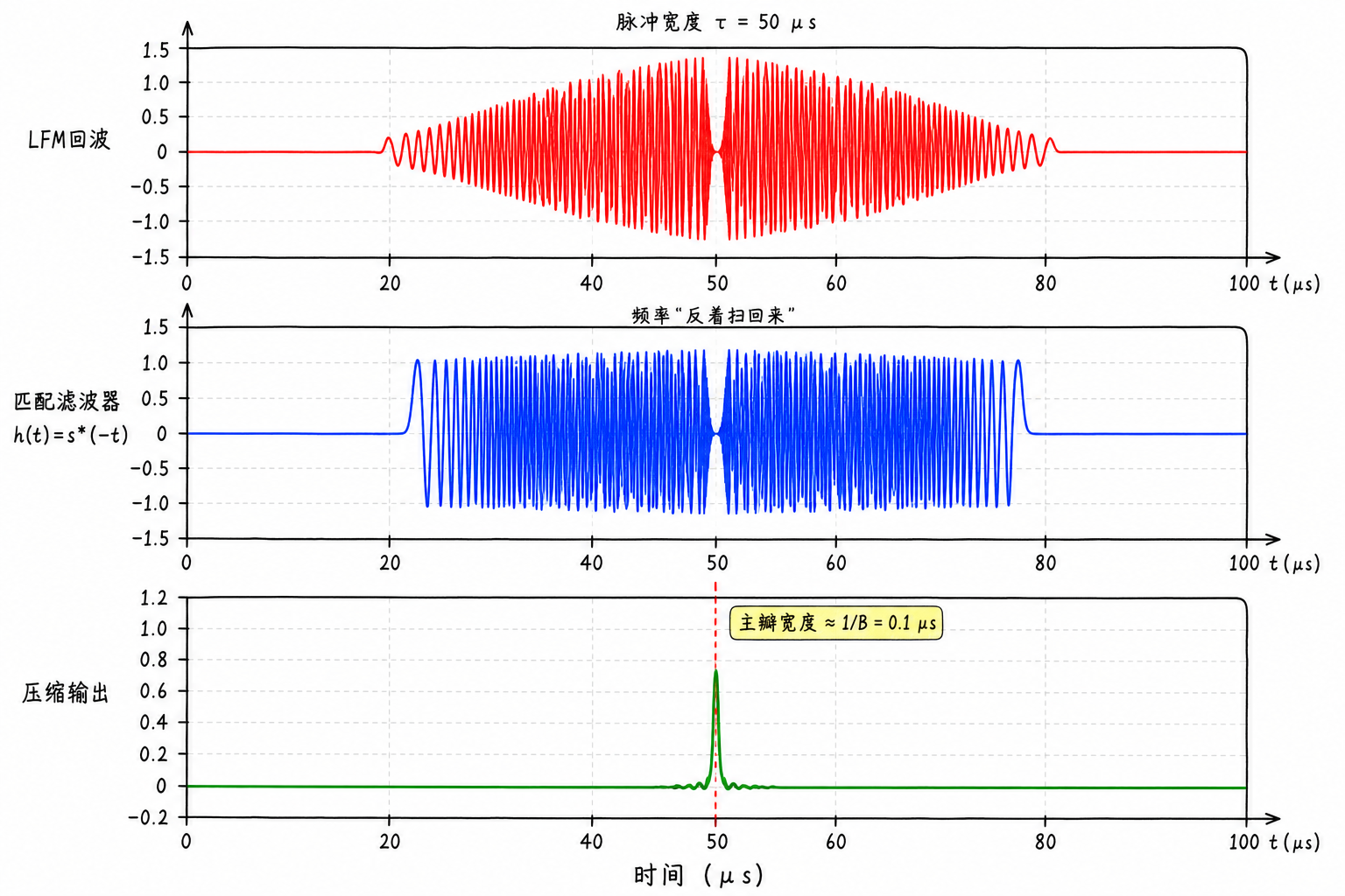
In Figure 4.14, the first row shows the received LFM echo, the second row shows the impulse response of the matched filter, and the third row shows the compressed output. The echo, originally tens of microseconds wide, is compressed into a much narrower mainlobe.
The compressed mainlobe width is approximately determined by $1/B$. If $B=10\,MHz$, the time mainlobe scale is about $0.1\,\mu s$, corresponding to a range scale of about $15\,m$. This is the same as the previously derived $\Delta R\approx c/(2B)$.
The matched filter output typically consists of a mainlobe and sidelobes on both sides, and is not equivalent to an ideal impulse.
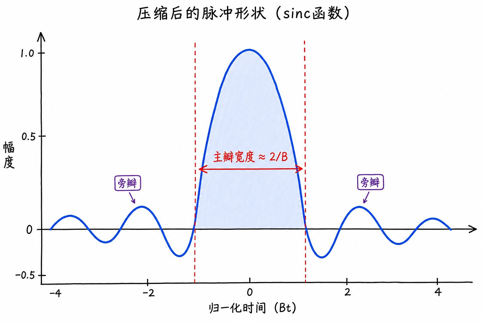
The highest part in the middle is called themain lobe, which determines the main position of the target peak and whether two targets can be separated. The fluctuations on both sides of the main lobe are calledsidelobes. Sidelobes are secondary peaks in the processing output caused by the waveform and filtering, and do not represent new targets.
Sidelobes affect visibility when strong and weak targets coexist. The sidelobes of a strong target may exceed the main lobe of a nearby weak target, making the weak target difficult to discern in the range profile.
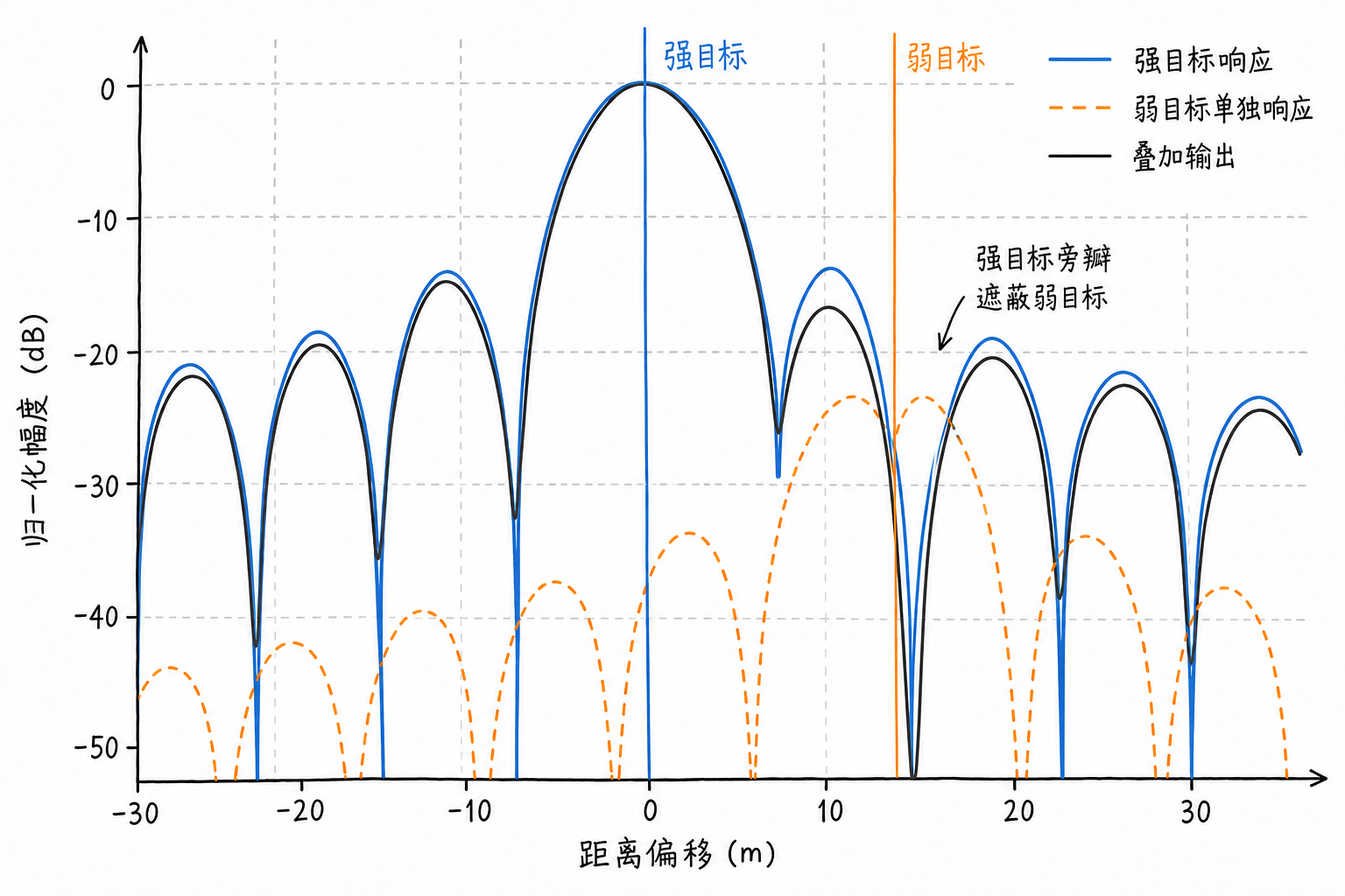
In Figure 4.16, the blue curve is the response from the strong target alone, the orange dashed line is the response from the weak target alone, and the black curve is the output after superposition. When the weak target is close to the strong target, it may fall near the sidelobes of the strong target, making the peak difficult to distinguish.
A common method to suppress sidelobes is windowing. Windowing can be understood as applying a smooth weight to the frequency domain or reference signal, softening abrupt edges to reduce sidelobes.
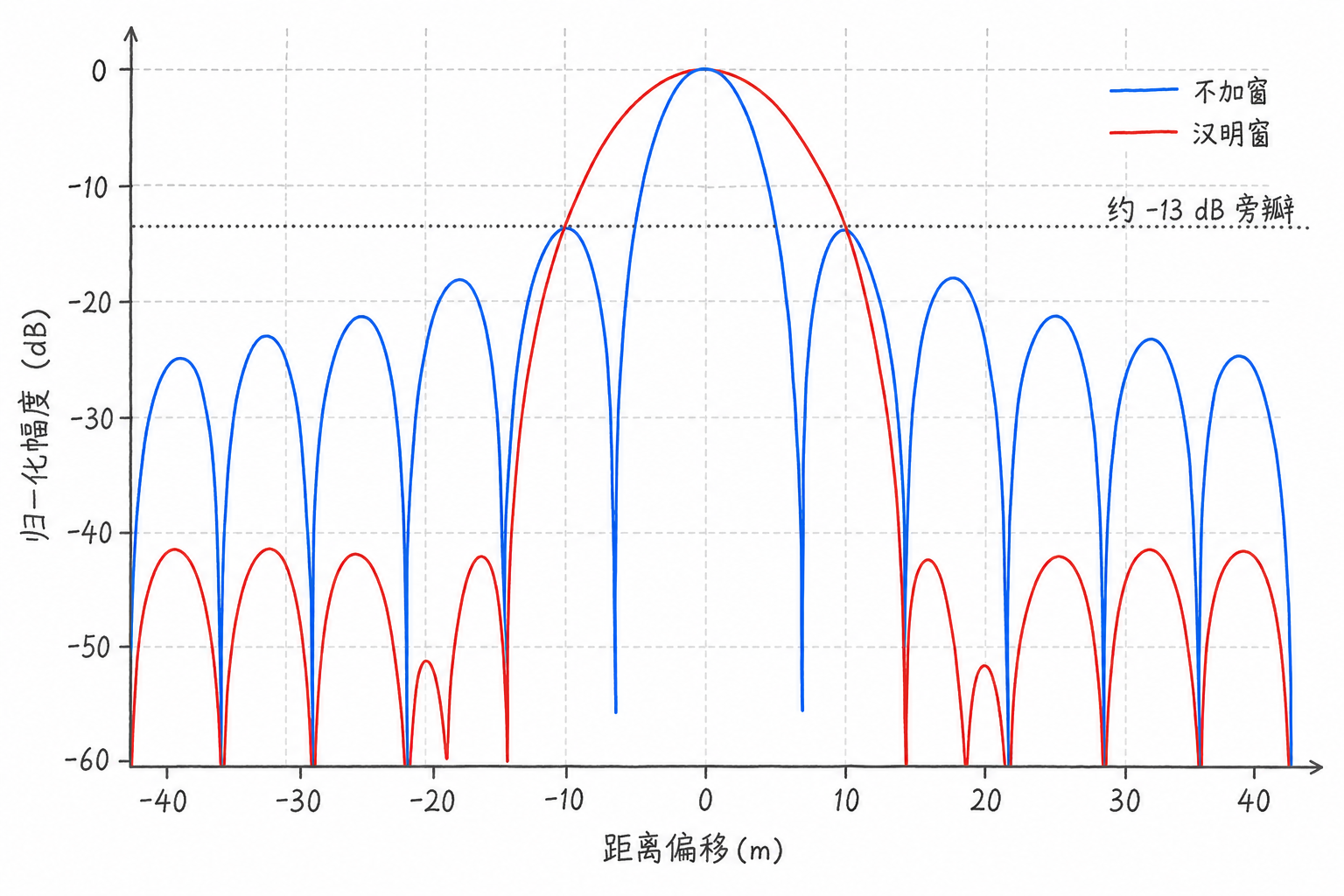
Windowing also has a cost. After reducing sidelobes, the main lobe typically widens, sacrificing range resolution. Engineering requires a tradeoff between two considerations: lower sidelobes favor detecting weak targets near strong ones; narrower main lobes favor separating adjacent targets.
4.5 Exercises
The following exercises combine several operations from Chapter 4: converting delay to range, observing SNR, distinguishing dual targets, changing bandwidth, and comparing main lobe and sidelobe changes caused by window functions.
Exercise 1: Single-Target Range Recovery
Consider a pulse radar using baseband LFM signal with the following parameters:
| Parameter | Value |
|---|---|
| Pulse width | $\tau=10\,\mu s$ |
| Bandwidth | $B=20\,MHz$ |
| Sampling rate | $f_s=100\,MHz$ |
| Target range | $R=15\,km$ |
Explain: How to generate the transmit signal, construct the delayed echo, perform matched filtering, and recover the target range from the peak position?
Solution: Derive the chirp rate from bandwidth and pulse width
Then obtain the round-trip delay from the target range
Delay the transmit signal by $\Delta t$ to get the echo $r(t)$, construct the matched filter $h(t)=s^*(-t)$, and compute
Find the peak position in the output $y(t)$. In implementation, the peak index typically includes fixed offsets from the receive window start and matched filter length; after removing these offsets, the echo delay $\Delta t_{\text{peak}}$ is obtained, then converted to range:
This exercise covers the complete range processing chain: from waveform to echo, from matched filter output to range axis.
Exercise 2: Varying SNR
If the SNR drops from $-10\,dB$ to $-20\,dB$, what happens to the peak in the matched filter output?
Solution: As SNR decreases, the noise floor rises and the contrast between the peak and background degrades. As long as the peak remains significantly above surrounding noise, it can still be detected; if noise fluctuations approach the peak level, range estimation and subsequent detection become unstable.
Exercise 3: Adding a Second Target
Add a second target at range $20\,km$ to the original single-target scenario. What changes occur in the range profile? If the two targets gradually move closer, when will they merge into a single peak?
Solution: Adding a second target produces a second peak in the matched filter output. If the range separation exceeds the system range resolution, they typically appear as two separable peaks; if the separation is less than the resolution, the two mainlobes overlap and the range profile may show only a single broadened or distorted peak.
Exercise 4: Varying Bandwidth
If bandwidth changes from $20\,MHz$ to $5\,MHz$, how does the peak width change?
Solution: The range resolution after pulse compression approximately satisfies
As bandwidth drops from $20\,MHz$ to $5\,MHz$, resolution degrades and the peak broadens. Two nearby targets merge more easily. This phenomenon connects the $B$ in the formula to the mainlobe width in the range profile.
Exercise 5: Applying Window Functions
What effects does applying a Hamming window in matched filtering have on mainlobe width and sidelobe level?
Solution: Windowing suppresses sidelobes, reducing secondary peaks near strong targets; however, the mainlobe typically broadens, sacrificing range resolution. Stronger windows are not always better—they reflect the tradeoff between sidelobe suppression and mainlobe width.