Chapter 6: Target Detection
6.1 What Does Target Detection Determine
Chapter 4 converted time delays in the echo into range, and Chapter 5 converted phase changes in the echo into velocity. At this point in the processing, a common misconception arises: doesn't a peak in the range profile or range-Doppler map indicate a target?
Real radar data is never this clean. Peaks don't come only from targets: noise raises small spikes, clutter forms large background fluctuations, and sidelobes adjacent to strong targets create structures that look like targets. If we declared a target for every bump, false alarms would be too numerous to be usable.
So Chapter 6 addresses a very practical decision problem: should we trust this peak or not?
Prior processing has already produced the range profile or range-Doppler map; detection performs another screening on this map: cells that pass the threshold are marked as 1, those that don't are marked as 0. The resulting binary map is called adetection maskordetection map. Only cells marked as 1 in the detection mask proceed to plot generation and target list processing.
From Detections to Decision
Detection decisions are clearest when viewed through a single range profile. Suppose after matched filtering, the amplitudes of 8 range bins in one segment are
The amplitude of the 5th bin is 4.7, much higher than the surrounding background. Such a peak typically resembles a target, because the surroundings are mostly around 1, while it suddenly rises to 4.7.
Now change the data slightly:
The 5th bin now has only 1.6. It's still higher than its surroundings, but this difference is no longer as reliable. It could be a weak target, or it could just be noise that happened to spike once. The difficulty in detection lies in these cells that are "not obvious enough, yet can't be casually dismissed."
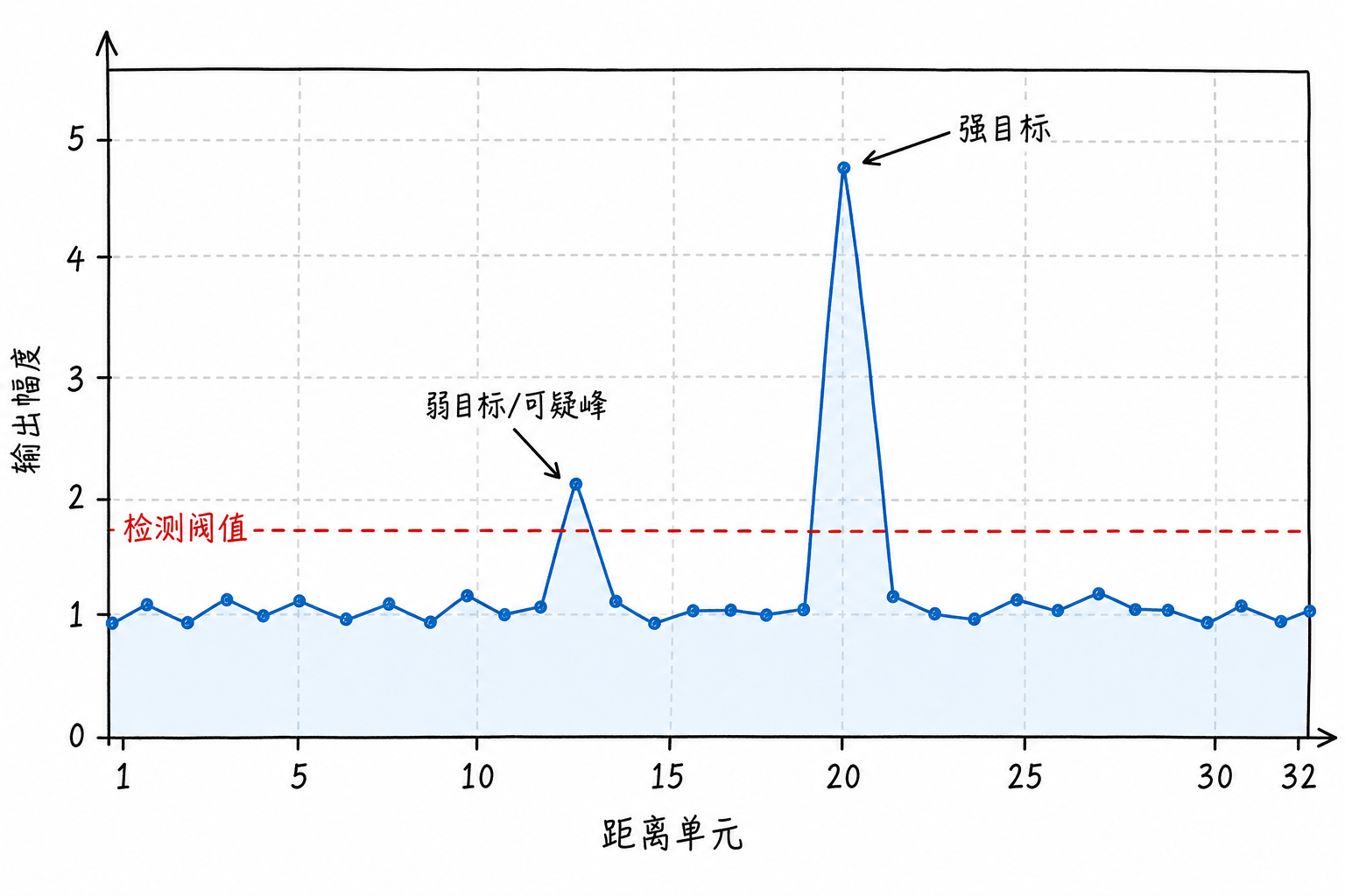
In Figure 6.1, strong targets are easy to identify; the boundary between weak targets and noise fluctuations is more ambiguous. The detection problem addresses another layer of task: among a pile of fluctuations, distinguishing which bumps are worth trusting and which are just background coincidentally spiking.
The same applies to the range-Doppler map. Each cell corresponds to a range and a velocity; the detector doesn't reinvent range and velocity, it only asks: is this cell's energy sufficiently trustworthy relative to the background? If trustworthy, it's marked as 1 in the detection mask; if not, it remains just a fluctuation on the map.
Two Detection Hypotheses
Actual receiver output cannot be completely clean. Even without targets, receiver thermal noise, ground clutter, sea clutter, sidelobes, and spectral leakage will cause some cells to have non-zero values. Therefore, the observed value in a detection cell can be understood as two cases.
When no target is present:
When a target is present:
Many textbooks formulate this as a binary hypothesis test:
Here $x$ is the observation in the current cell, $n$ denotes background noise or clutter, and $s$ denotes the target signal. $H_0$ represents "background only," and $H_1$ represents "target superimposed on background."
This notation looks formal, but the meaning is quite straightforward: is this value merely a background fluctuation, or is a target truly superimposed on the background?
Finding only local maxima cannot answer this question. For example
The 3rd cell is indeed higher than its neighbors, but it may not be a true target. A local maximum only indicates it is the peak within this small segment, not that it is high enough to be credible. Detection also requires a decision criterion.
Threshold Detection Rule
The most basic decision criterion is a threshold. Let the amplitude of the current cell be $x$ and the threshold be $T$. If
declare a target; if
do not declare a target. Written as a decision rule:
If we express the detector output as a function, it can be written as
where $\delta(x)=1$ indicates the cell is marked as a target, and $\delta(x)=0$ indicates no target is declared. Applying this decision cell-by-cell to an entire range profile or range-Doppler map yields a detection mask.
This rule appears straightforward, but it already carries a cost. Set the threshold too low, and noise easily masquerades as targets; set it too high, and weak targets slip through. Fixed thresholds, CFAR, and more complex statistical detection methods all ultimately convert a continuously varying observation into a binary "detect" or "no detect" decision. The main differences lie in how the threshold is derived, how the background is estimated, and how much false alarm and missed detection one is willing to tolerate.
6.2 Detection Threshold and Fixed Threshold Detection
The previous section compressed the detection problem into a single question: how large must a cell's output value be to qualify as a target? This "how large" is the threshold.
The threshold appears to be just a number, yet it determines the detector's stance: whether to favor reporting liberally and miss nothing, or to remain conservative and avoid false alarms.
Fixed Threshold Detection
If the background is relatively stable, start with a constant as the threshold. Suppose that during a period without targets, range cell amplitudes typically fluctuate between 0.6 and 1.4. Setting the threshold to $T=2.0$ means values exceeding 2.0 are reported as targets, and those below are not. This is fixed-threshold detection.
The rule remains
where $T$ is a preset constant. If the background hovers around 1 for extended periods, fluctuations like 1.1 or 1.2 typically aren't worth reporting; a cell suddenly reaching 4 or 5 looks much more like a target. The value of a fixed threshold lies in providing a baseline ruler that makes the detection action repeatable.
For example, if $T=2.0$ and a cell outputs $x=4.7$, then because
it is judged as a target. If a cell outputs $x=1.1$, then because
it is judged as no target. Such judgments are typically uncontroversial.
Trouble arises in edge regions. If a cell outputs $x=1.9$, by the rule
it is still judged as no target. But 1.9 is already noticeably higher than the background—it could be a weak target or merely background fluctuation. A fixed threshold compresses complex judgment into a single number; the advantage is simplicity, the cost is sensitivity in edge cases.
Consequences of Threshold Levels
Lowering the threshold makes weak targets easier to detect, but noise also crosses the threshold more easily. Consider a data set with no targets present:
If the threshold is $T=2.0$, this data set will not trigger an alarm. If the threshold is lowered to $T=1.3$, both 1.4 and 1.5 will trigger alarms. The problem is that, by assumption, no targets are present—the alarms are entirely caused by background fluctuations.
Conversely, raising the threshold reduces false alarms, but weak targets are more easily missed. Suppose a weak target produces a cell output of $x=2.8$. When the threshold is $T=2.0$,
it can be detected. If the threshold is raised to $T=3.5$, then
it will be classified as no target.
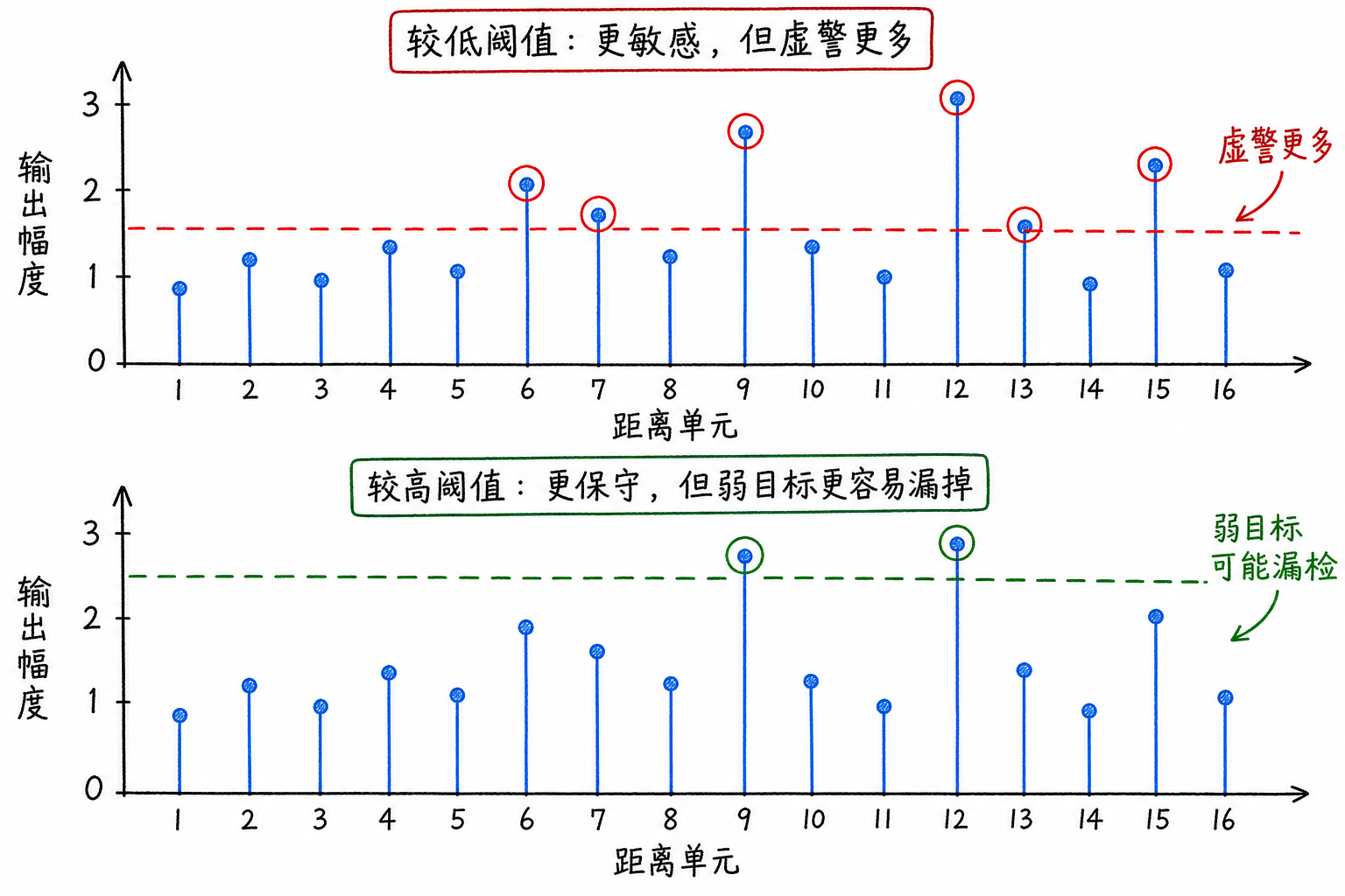
Figure 6.2 shows the results for the same data under different thresholds. With a low threshold, more cells trigger alarms, some of which may be merely background. With a high threshold, fewer cells alarm, but weak targets may also fall below the threshold. The detector faces a tradeoff from the start: be conservative or be sensitive.
Background Limitations on Fixed Thresholds
A fixed threshold also assumes the background level does not vary too widely. If the background is roughly uniform across the entire map, a constant threshold may still work. In real radar maps, the background often varies with range, azimuth, velocity cell, or environmental conditions.
For example, in the same range profile there are two regions. Region A has a background roughly around 1:
With a fixed threshold $T=2.0$, the 2.6 in the middle will be detected. Region B has an elevated background around 4 to 6:
Using the same $T=2.0$, nearly the entire region will alarm. Region B does not have targets everywhere; the problem is that the threshold is below the background level in that area.
If the fixed threshold is raised to 6.0to accommodate Region B, some real but weak targets in Region A may be missed. A single global constant can hardly adapt to both clean regions and clutter regions simultaneously. Fixed thresholds are suitable for building initial intuition and for simplified scenarios with stable backgrounds; when the background varies significantly, the threshold needs to adjust with the local background.
6.3 False Alarms, Missed Detections, and Detection Performance
As seen in the previous section, the threshold cannot be both low and high at the same time. When the threshold is lowered, weak targets are more easily detected, but noise also crosses the threshold more easily. When the threshold is raised, false alarms decrease, but weak targets are also more easily blocked.
In engineering practice, one cannot design a detector based solely on 'feels about right'; explicit metrics are needed to describe detection performance: how frequently false alarms occur, and how likely it is to miss a target.
False Alarm Rate, Missed Detection Rate, and Detection Probability
These two types of errors cannot be discussed together.
When the detector reports 'target present' when there is actually no target, this is called afalse alarm. In a large number of no-target tests, the proportion of false alarms is called thefalse alarm rate, denoted as $P_{FA}$.
When a target is actually present but the detector fails to report it, this is called amiss. The miss probability is commonly denoted as $P_M$. Correspondingly, when a target is actually present and the detector successfully reports it, the probability is called thedetection probability, denoted as $P_D$. When a target is present, it is either detected or missed, so
Consider a counting example. A radar operates 100 times under target-free conditions, and alarms are triggered 8 times. Then the
false alarm rate is 8%. Next, the radar operates 100 times under target-present conditions, successfully reporting the target 83 times and failing to report it 17 times. Then
These metrics decompose "detection performance" into comparable quantities. A detector may have few false alarms but many misses, or high detection rate but many false alarms. Simply saying "looks acceptable" is insufficient—at minimum, one must state what detection probability it achieves at a given false alarm level.
Threshold Trade-offs and ROC Curves
Suppose background noise amplitude is mostly distributed between 0 and 2, while weak target signals superimposed on background are mostly distributed between 1 and 3. The two ranges overlap: some larger noise samples reach 1.8 or 1.9, while weaker target samples may only be 1.5 or 1.7.
Whenever two sample classes overlap, no perfect decision boundary exists. Setting the threshold at 1.2 allows many targets to be detected, but many noise samples will also cross the line; setting the threshold at 2.5 reduces false alarms, but some weak targets will also be blocked.
| Threshold | Detection probability $P_D$ | False alarm rate $P_{FA}$ |
|---|---|---|
| 1.2 | 0.97 | 0.22 |
| 1.8 | 0.88 | 0.08 |
| 2.5 | 0.65 | 0.01 |
The table shows that when the threshold is set to 1.2, detection probability is high but false alarm rate is also high; when the threshold is set to 2.5, false alarm rate is low but detection probability also drops; a threshold of 1.8 lies in the middle. Such tables are very useful in engineering because they present the tradeoff between "sensitivity" and "reliability" in a single view.
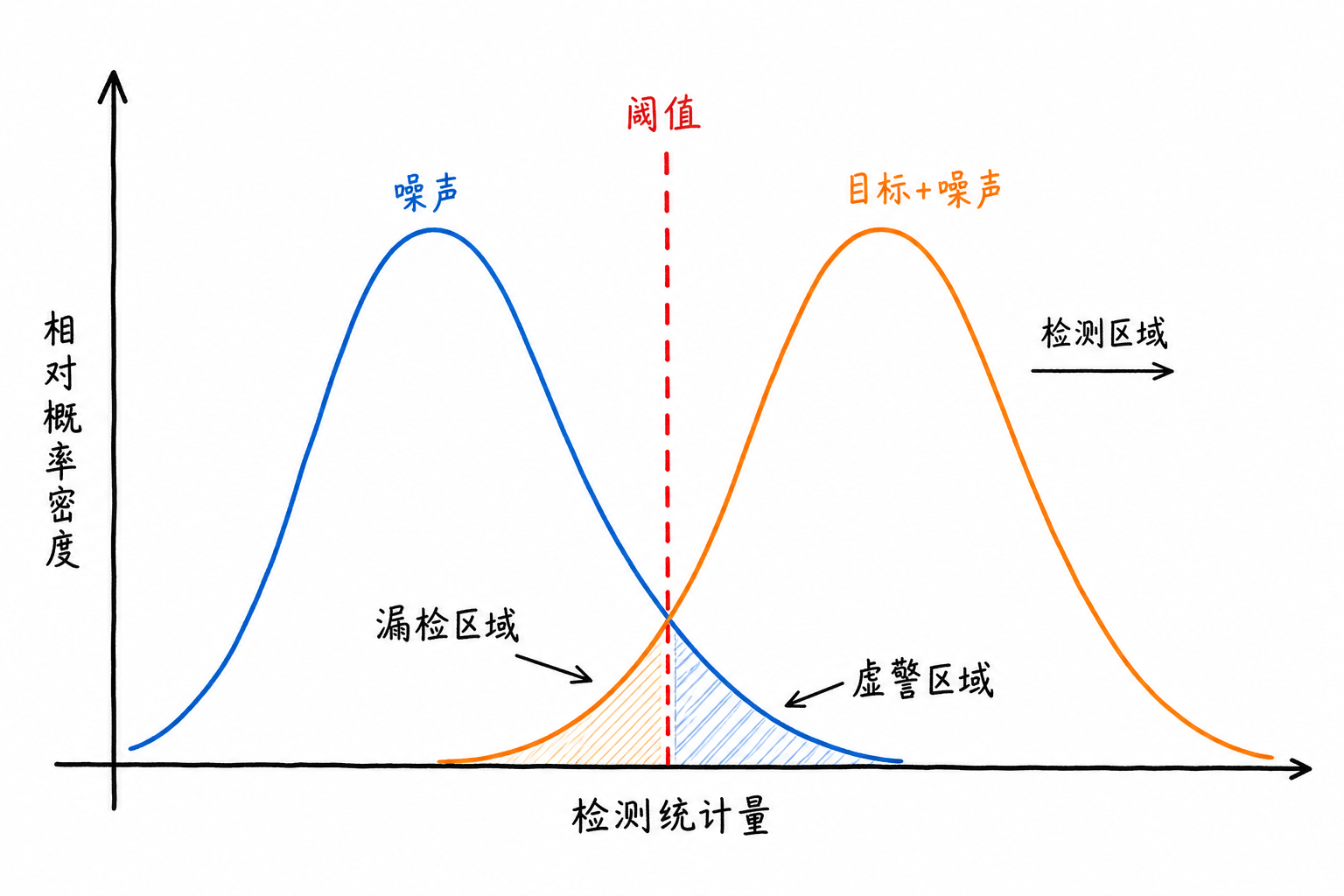
Figure 6.3 illustrates this dilemma using two distributions. The blue region represents background noise, and the orange region represents the output after a target is superimposed on the background. Moving the threshold left allows more targets to exceed it, but also more noise; moving it right reduces false crossings by noise, but also makes weaker targets easier to miss.
Connecting the $(P_{FA}, P_D)$ points corresponding to different thresholds produces the ROC curve.
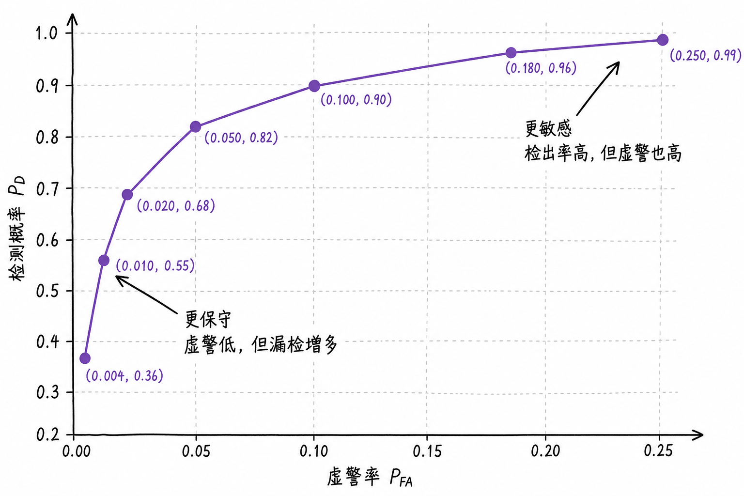
The ROC curve plots false alarm rate on the horizontal axis and detection probability on the vertical axis. A curve closer to the upper left indicates that high detection probability can be maintained even at low false alarm rates. When starting out, there's no need to derive the statistical origins of the ROC—focus first on reading it: the same detector operating at different thresholds moves along the curve; achieving higher $P_D$ typically requires accepting higher $P_{FA}$.
False Alarm Constraints and SNR
Real systems often begin by specifying an acceptable false alarm level. For example, allowing on average only 1 false alarm per 1000 target-free cells, or ensuring the number of false alarms in each range-Doppler map doesn't overwhelm downstream processing. With such requirements established, the threshold is then selected accordingly.
This is the idea behind "designing the threshold based on false alarm rate." Complete detection theory further discusses the Neyman-Pearson criterion: maximizing detection probability under a given false alarm rate constraint. This book retains that background but does not develop the likelihood ratio test derivation.
Another quantity affecting detection difficulty is signal-to-noise ratio (Signal-to-Noise Ratio, SNR). In power form it can be written as
where $P_s$ is the target signal power and $P_n$ is the noise power. When SNR is high, target samples and background samples separate more easily; when SNR is low, the two classes overlap more, and the same threshold more readily produces both false alarms and missed detections.
The threshold makes the decision; SNR determines how difficult that decision is. If the target itself is weak and the background is strong, no amount of threshold adjustment can eliminate all errors. What a detector can do is maximize detection capability at an acceptable false alarm level.
A fixed threshold imposes this tradeoff on a single global value. If the background across the entire map is stable, this value can work; if the background rises or falls in different regions, the same threshold will be too low in some places and too high in others. CFAR is designed precisely for this situation.
6.4 Constant False Alarm Rate Detection (CFAR)
When discussing thresholds in previous sections, there has been a hidden assumption: the background is roughly stable. Only under this assumption does a fixed threshold work like a universal ruler that can be applied anywhere with roughly consistent results.
Real environments are rarely like this. Clutter may be stronger at close range, the noise floor may be lower at long range, terrain, sea waves, or rain cells may exist in certain directions, and fluctuation levels in different regions of the range-Doppler map can vary dramatically. A fixed threshold easily produces this result: too high in quiet regions, too low in noisy regions.
From Fixed Threshold to Adaptive Threshold
CFAR stands for Constant False Alarm Rate, commonly translated asconstant false alarm rate. Its starting point is to change the threshold from a hard-coded constant to a quantity that automatically adapts based on the surrounding background.
Look again at the two regions from before. Region A has a background around 1, and the center value of 2.6 does stand out considerably; Region B has a background around 5, and the center value of 5.8 is not prominent. If a fixed threshold $T=2.0$ is used, Region B will trigger many alarms. If each position first examines the nearby background and then sets the threshold to some multiple of that background, Regions A and B will receive different thresholds.
This process can be summarized in three steps: first estimate the background level near the current cell, then leave headroom according to the target false alarm rate, and finally compare the current cell against this local threshold.
On a one-dimensional range profile, it appears as a sliding window; on a two-dimensional range-Doppler map, it appears as a neighborhood window surrounding a given cell. The following uses a one-dimensional window for illustration, as it makes the roles of the CUT, guard cells, and reference cells easiest to see.
CUT, Guard Cells, and Reference Cells
The current cell being judged is called theCell Under Test, commonly written as CUT (Cell Under Test). Suppose a sequence of data is
The center value of 3.2 is the CUT. If the surrounding 6 cells are used to estimate the background, the mean is
If the threshold is set to 3 times the background estimate, then
The CUT is 3.2, satisfying
so it is judged as a target. This example already contains the main actions of CFAR: local background estimation, local threshold generation, and local decision making.
In real processing, cells immediately adjacent to the CUT cannot be used for background estimation. Target responses usually don't land in just one cell; mainlobe edges and sidelobes may affect nearby cells. If these cells participate in averaging, the background estimate will be elevated by target energy, the threshold will rise accordingly, and weak targets become more likely to be missed.
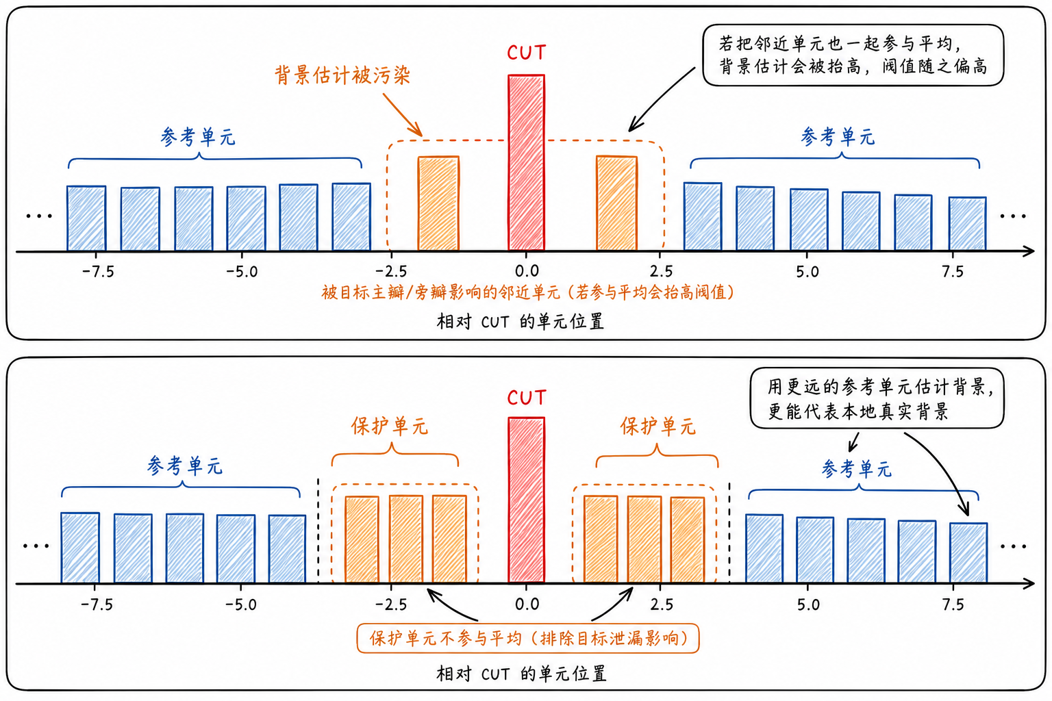
Therefore, on both sides of the CUT, there will beGuard Cells(Guard Cells). Guard cells do not participate in background estimation; they only serve to separate the CUT from the reference region. A set of cells farther away are calledReference Cells(Reference Cells), used to estimate the local background.
The window for one-dimensional CA-CFAR can be written as
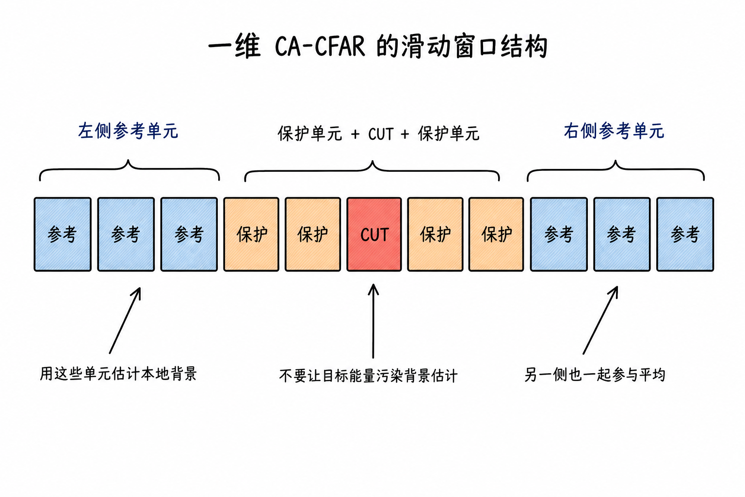
Guard cells answer "which locations may already be affected by the target and are unsuitable for background estimation"; reference cells answer "how high the background is in this region". Once these two roles are clarified, the CFAR window structure becomes straightforward.
CA-CFAR Computation and Limitations
The most basic type of CFAR is CA-CFAR, where CA stands for Cell Averaging. It estimates the background power or amplitude using the average of the reference cells, then multiplies by a threshold factor to form a local threshold.
In power form, this can be written as
where $\hat P_n$ is the local background estimated from the reference cells, and $\alpha$ is the threshold factor. Then compare
$\alpha$ cannot be omitted. If the threshold only equals the background average, slightly higher fluctuations in the background can easily cross the line, resulting in many false alarms. $\alpha$ provides a safety margin: the larger $\alpha$ is, the higher the threshold, the fewer false alarms, but weak targets also become harder to detect. The rigorous relationship between $\alpha$ and $P_{FA}$ requires assuming a background distribution, which this book does not derive in detail.
Consider a simplified calculation. The CUT power is 12, and the reference cell powers on both sides are
The reference cell average is
If $\alpha=2$, then
Since
the CUT is declared as a target.
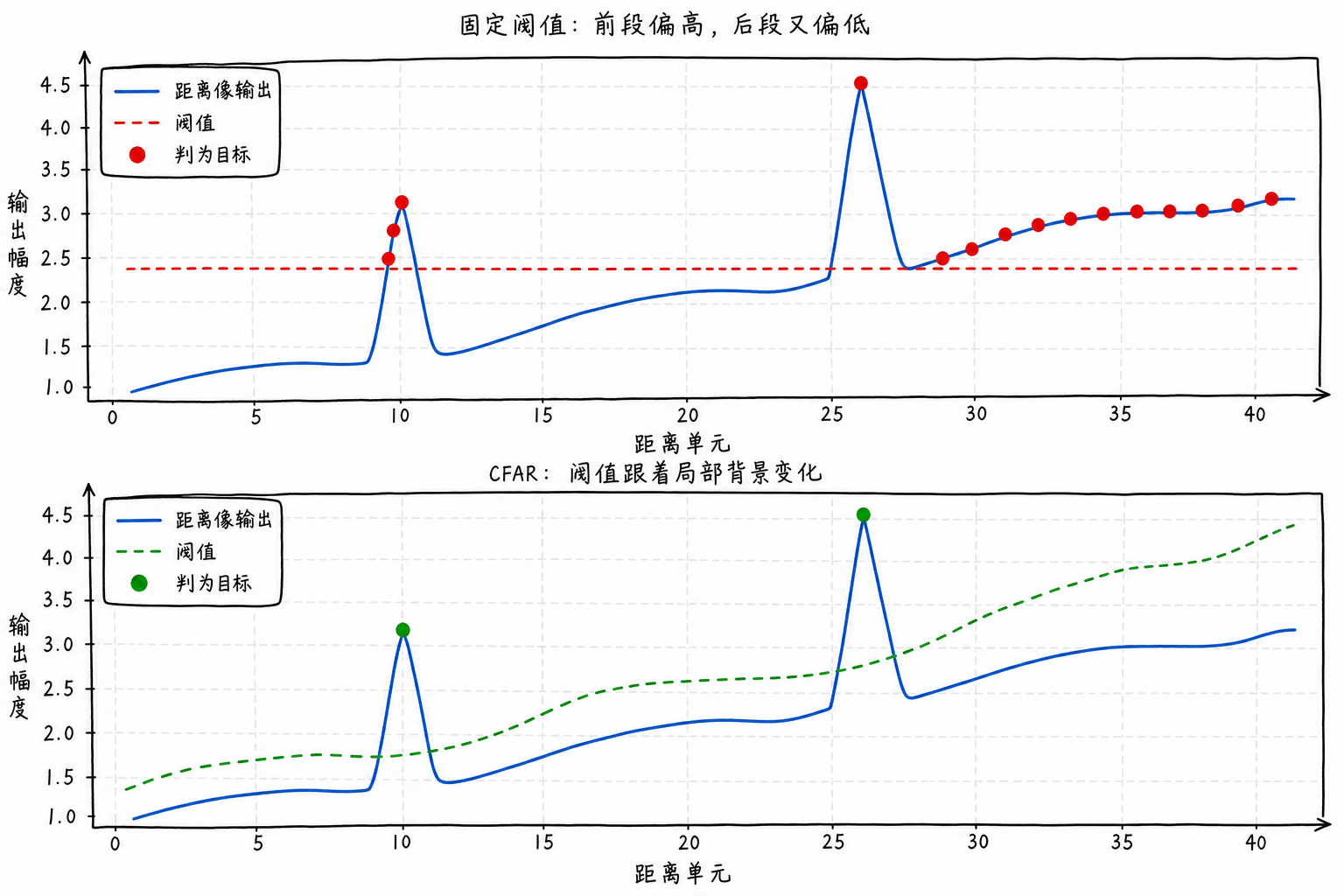
Figure 6.7 compares fixed threshold and CFAR on the same range profile with non-uniform background. The fixed threshold is a horizontal line that easily produces consecutive false alarms when the background rises; the CFAR threshold follows local background variations, providing different thresholds in different regions.
CA-CFAR also has limitations. It assumes reference cells represent the local background. If another strong target contaminates the reference cells, the average will be elevated and weak targets may be missed; if the window straddles a clutter edge with high background on one side and low on the other, simple averaging may not be appropriate; when targets are dense, reference cells can hardly maintain pure background.
These limitations do not overturn the CFAR framework. The CUT, guard cells, and reference cells still exist; the change mainly occurs in how to estimate background using reference cells.
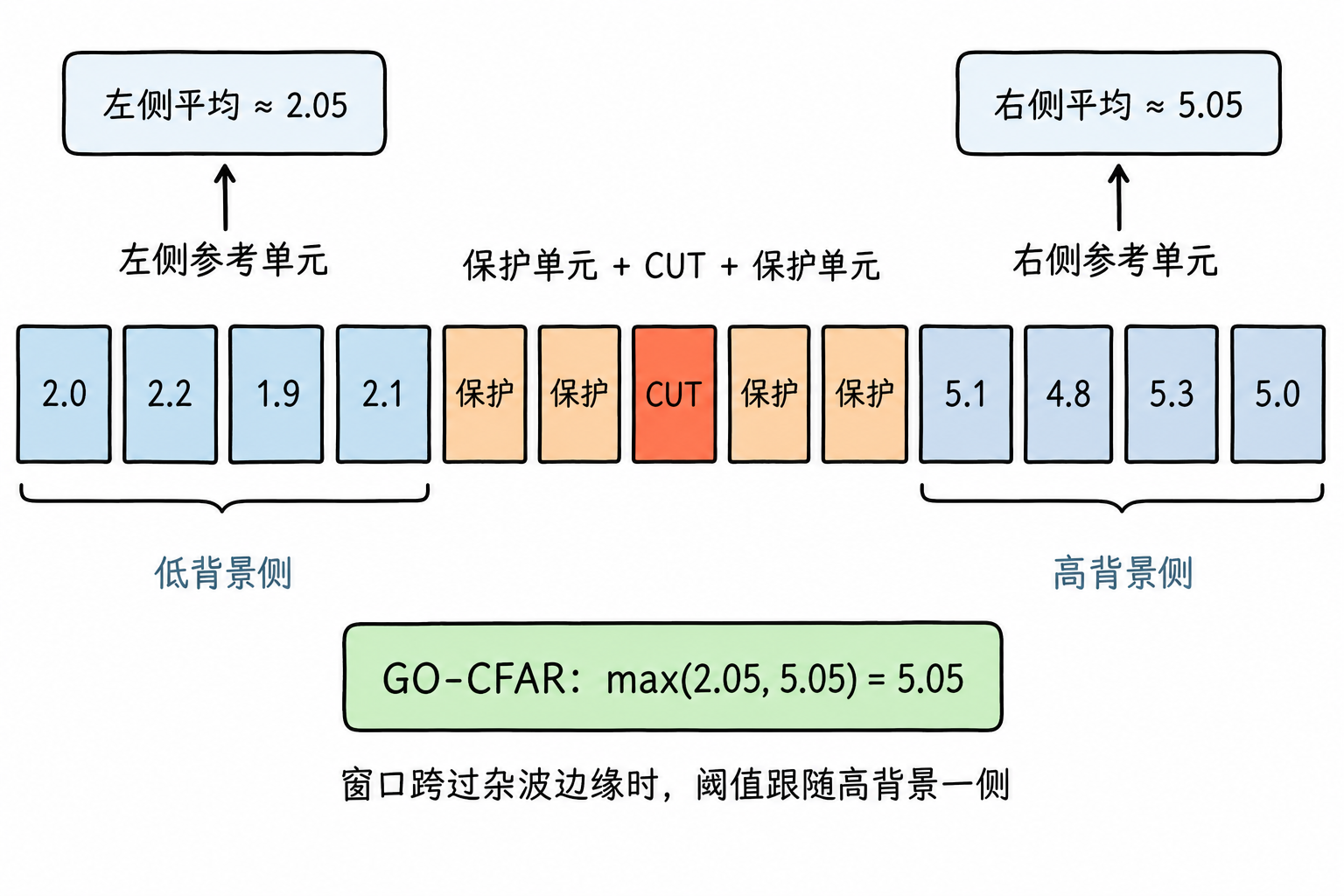
One common variant is GO-CFAR, where GO stands for Greatest Of. It computes the reference cells on the left and right sides of the CUT separately—calculating an average on the left and another on the right—then takes the larger of the two as the background estimate. This approach is conservative: if the window straddles a clutter edge, the high-background side raises the threshold, reducing false alarms near clutter edges. The cost is that the threshold may be too high, making weak targets near high-clutter regions more easily missed.
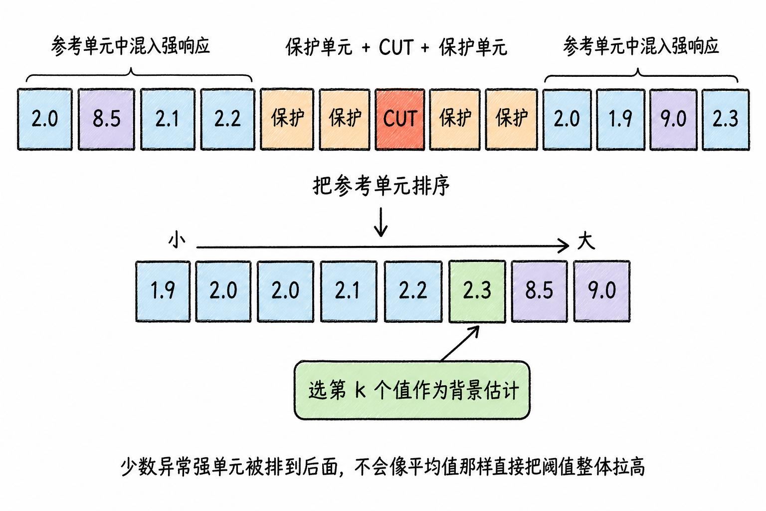
Another common variant is OS-CFAR, where OS stands for Ordered Statistic. It first sorts the reference cell values in ascending order, then selects the value at a certain rank position as the background estimate. The advantage is that one or two exceptionally strong reference cells do not elevate the threshold as much as averaging would, so OS-CFAR is commonly used when targets are dense and the reference window is easily contaminated by other targets. The cost is an additional rank position parameter; choosing a higher position makes detection more conservative, while choosing a lower position may lead to more false alarms.
Therefore, CA-CFAR is suitable for introductory scenarios with relatively uniform backgrounds; GO-CFAR emphasizes suppressing false alarms at clutter edges; OS-CFAR emphasizes maintaining stable background estimation under multi-target or outlier contamination. They address different problems, but all do the same thing: first estimate the background around the CUT, then compare the current cell against a local threshold.
6.5 Plot Aggregation: From Detection Cells to Target Plots
After making cell-by-cell decisions with a fixed threshold or CFAR, the system obtains a detection mask: which range cells and velocity cells passed the detection threshold. But each 1 in this binary map does not necessarily represent an independent target.
If reported cell by cell, the same car, aircraft, or rain cluster could be split into multiple targets. Here we first understand a plot as a candidate target record; plot clustering handles the post-detection consolidation work: merging or filtering adjacent alarms to form target plots that are easier for downstream processing to use.
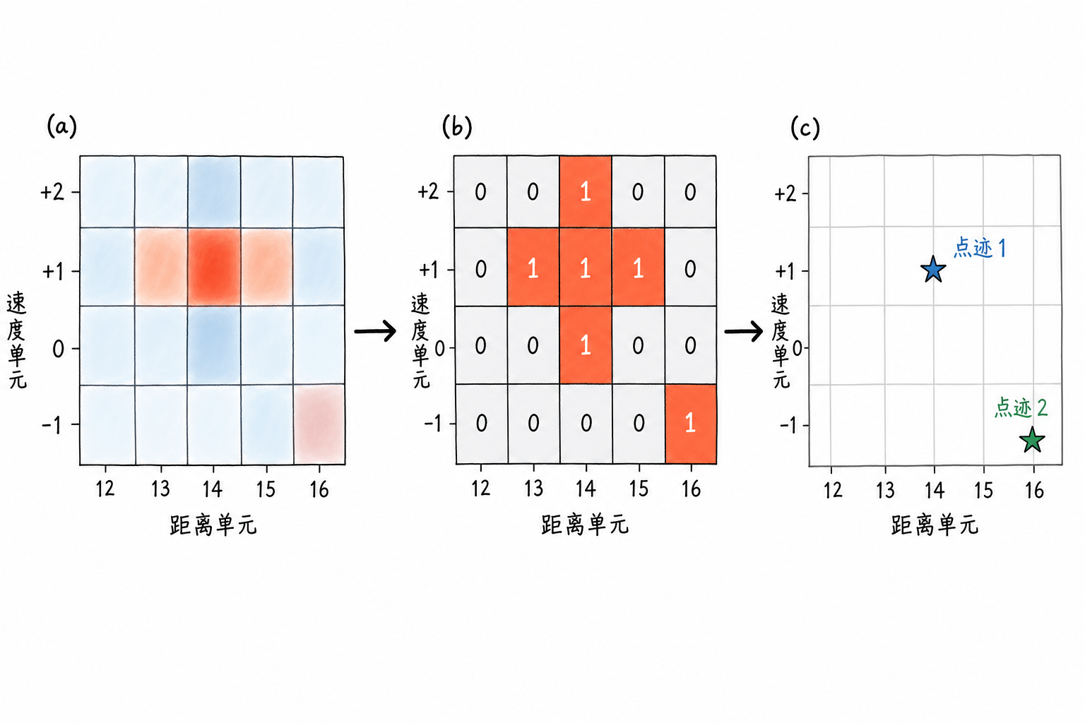
Figure 6.10 shows these three layers together: the range-velocity map preserves continuously varying response magnitude; the detection mask retains only positions above threshold; plot clustering then consolidates adjacent alarms into a small number of candidate target records.
Why a target lights up a patch of cells
An ideal point target can be thought of as falling into only one range-velocity cell; actual range-velocity maps are often wider. The mainlobe after pulse compression has width, the spectral peak after FFT also has width, and windowing functions, sidelobes, target extent, and grid position all cause energy to spread to nearby cells. As long as nearby cells also exceed the threshold, they will all become 1 in the detection mask.
For example, the detection result in a local range-velocity region is:
| Velocity bin / Range bin | 12 | 13 | 14 | 15 | 16 |
|---|---|---|---|---|---|
| +2 | 0 | 0 | 1 | 0 | 0 |
| +1 | 0 | 1 | 1 | 1 | 0 |
| 0 | 0 | 0 | 1 | 0 | 0 |
These 5 detection cells are very likely from the same target's response, not 5 targets arranged in a cross pattern. Without clustering, the target list would be filled with duplicate alarms, interfering with subsequent display, track processing, and manual interpretation.
Therefore, the first step after detection is to see whether adjacent alarms belong to the same candidate region, then decide how to report them.
Connected regions, local peaks, and plot parameters
An intuitive approach is to first findconnected regions. In a1D range profile, adjacent range cells that are consecutively 1 can be treated as a group; in a 2D range-velocity map, detection cells adjacent in range or velocity direction can also be grouped together. In engineering implementation, 4-connectivity or 8-connectivity can be used; at the introductory stage, just grasp one point: alarms that are next to each other are first treated as a candidate target region.
After finding a region, a representative position must be selected. A simple rule is to take the cell with the maximum original magnitude or power as the peak point of this region. For the cross-shaped region above, if the strongest response appears at range bin 14, velocity bin +1, the plot position can be recorded as this cell, along with magnitude, SNR, region size, and other information.
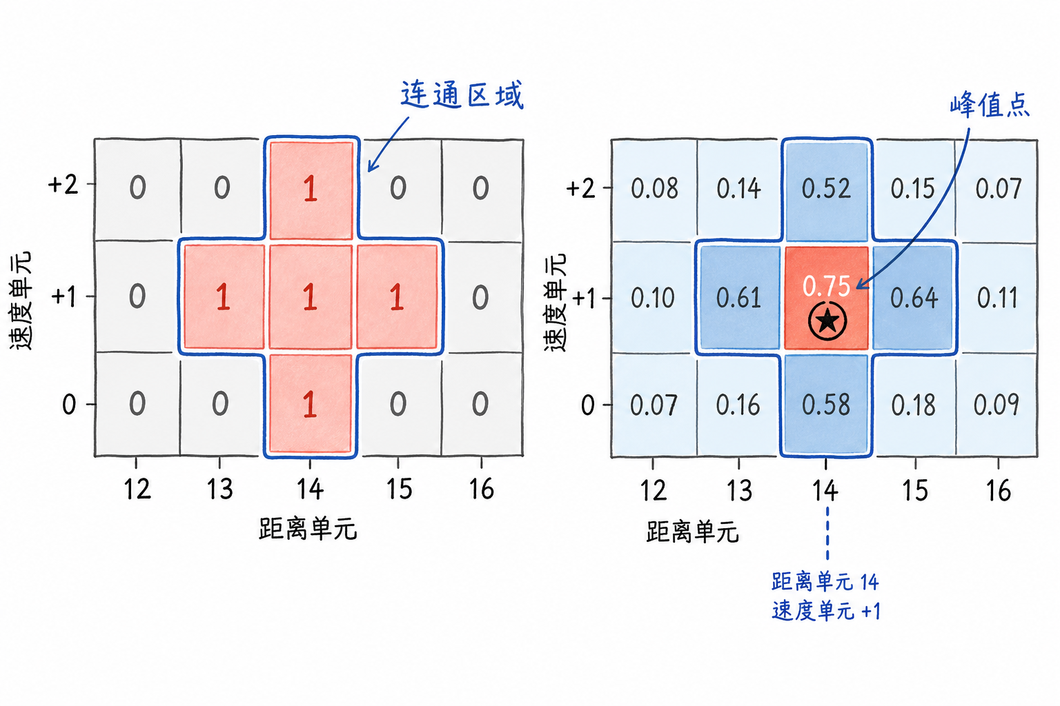
Figure 6.11 The left side shows adjacent alarms in the detection mask, while the right side places the original response magnitudes back into the same region. The strongest cell within the region is selected as the peak point, and its position becomes the representative position for this plot.
Some systems do not explicitly find connected regions first, but instead performlocal peak filtering: a detection cell is retained only if it appears more peak-like than neighboring cells in both the range and velocity directions. This approach is not contradictory to the connected-region method. Both aim to avoid repeatedly reporting multiple alarms from the vicinity of the same target.
In radar, this type of detection report is commonly called aplot. This name can be understood by breaking it down: after clustering, it manifests as a representative position in the current frame of data, hence it is a "point"; this point comes from a single observation and is the detection record left by the target in this frame, hence called a "trace." A plot emphasizes the candidate target position left by a single-frame observation.
A plot typically records its range bin, velocity bin, converted physical range and radial velocity, and also records the amplitude or SNR to indicate how strong this plot is. Real systems may also record fields such as target region width, beam number, timestamp, etc.
Plot clustering also involves trade-offs. If clustering is too aggressive, two targets that are close in range or velocity may be merged into a single plot; if clustering is too weak, one target may be split into multiple plots. Therefore, clustering rules must be considered together with range resolution, velocity resolution, CFAR window, and target scenarios.
Plots are only single-frame detection results, not yet tracks. Tracks require associating plots across multiple frames and then estimating target motion state. In the processing chain of this chapter, the range-velocity map produces response magnitudes, detection produces the detection mask, and plot clustering organizes adjacent alarms into target plots.
6.6 Exercises
Exercise 1: Fixed threshold detection
A range bin outputs amplitude $x=2.7$, and the fixed threshold is $T=2.0$. Should this cell be judged as target present or target absent?
Solution: Compare the current cell with the threshold. Because
target present is declared. This exercise corresponds to the detector's first action: converting continuous values into discrete decisions.
Exercise 2: Consequences of raising the threshold
A weak target's cell outputs $x=2.4$. How does the detection result change when the threshold is raised from $T=2.0$ to $T=2.8$?
Solution: When $T=2.0$,
The cell is determined to contain a target. After raising the threshold to $T=2.8$,
the result changes to no target detected. Increasing the threshold reduces some false alarms but also makes weak targets easier to miss.
Exercise 3: False alarm rate, detection probability, and miss rate
A detector reports 6 false alarms in 200 target-free tests; it successfully detects 129 out of 150 target-present tests. Find $P_{FA}$, $P_D$, and $P_M$.
Solution: The false alarm rate is
The detection probability is
The miss probability is
Therefore, the false alarm rate is 3%, the detection probability is 86%, and the miss probability is 14%.
Exercise 4: Fixed threshold under varying background
In the same range profile, the background in region A fluctuates around 1, while the background in region B fluctuates around 5. If a fixed threshold $T=3$ is uniformly applied, what differences will occur between the two regions?
Solution: In region A, the threshold of 3 is well above the background, so false alarms will be minimal—only significantly elevated peaks will trigger detection. In region B, the background already fluctuates around 5, so the threshold of 3 falls below much of the background variation, triggering many false alarms. A fixed threshold assumes the background is roughly uniform across the entire scene; when the background is non-uniform, performance becomes imbalanced.
Exercise 5: A simplified CA-CFAR calculation
In a one-dimensional range profile, the Cell Under Test (CUT) has a power of 12. The reference cell powers are
Guard cells are skipped and do not participate in the calculation. If the threshold factor is $\alpha=2$, is this cell determined to be a target?
Solution: First calculate the reference cell average:
The local threshold is
Finally, compare the CUT with the threshold:
Therefore, this cell is determined to contain a target.
Exercise 6: The role of guard cells
What problems might occur if cells immediately adjacent to the CUT are also included in the reference cell average?
Explanation: If a target is indeed present near the CUT, energy from the target's mainlobe edges or sidelobes may leak into adjacent cells. Using these cells to estimate the background would raise the background average, and the threshold would rise accordingly. A weak target that should have been detected might then fall below the threshold. Guard cells are used to reduce this contamination of the background estimate by target energy.
Exercise 7: CA-CFAR failure scenarios
Imagine two strong targets are very close together, or reference cells on one side fall within a strong clutter region. What difficulties might simple CA-CFAR encounter?
Explanation: CA-CFAR relies on reference cells to estimate the local background. When two strong targets are close together, reference cells may contain another target, raising the average; when the window crosses a clutter edge, reference cells on one side cannot represent the background on the other side. Both situations cause the threshold to deviate from the true background near the current CUT, potentially leading to missed detections or false alarms. This is why variants like GO-CFAR and OS-CFAR have been developed in practice.
Exercise 8: From range-Doppler map to detection mask
Assuming a range-velocity map has been obtained in Chapter 5, describe how to use a fixed threshold or simplified CA-CFAR to obtain a detection mask, and explain what a1 in the mask represents.
Explanation: The fixed threshold approach compares the amplitude or power at each cell in the range-velocity map: positions exceeding the threshold are set to 1, otherwise to 0. The simplified CA-CFAR approach processes each cell as a CUT, leaves guard cells around the CUT, uses reference cells to estimate the local background and generate a local threshold, then compares the CUT against the threshold.
A1 in the detection mask indicates that the cell has passed the detection threshold and can be treated as a candidate target for further processing. It is not yet a complete target list; the cell indices still need to be converted to range and velocity coordinates, and plot clustering must handle issues like merging adjacent cells and peak selection.
Exercise 9: From detection mask to plots
A local detection mask is shown below:
| Row / Column | 1 | 2 | 3 | 4 | 5 |
|---|---|---|---|---|---|
| 1 | 0 | 0 | 0 | 0 | 0 |
| 2 | 0 | 1 | 1 | 0 | 0 |
| 3 | 0 | 1 | 1 | 0 | 0 |
| 4 | 0 | 0 | 0 | 0 | 1 |
If plot clustering is performed based on adjacent cell connectivity, roughly how many plots will this mask form? If the original amplitude is highest at row 2, column 3 in the upper-left region, how can its representative position be selected?
Explanation: The 4 ones in the upper-left are adjacent to each other and should first be treated as one candidate region; the 1 in the lower-right is separate and should be treated as another region. Therefore, this local mask roughly forms 2 plots.
If row 2, column 3 has the highest amplitude in the upper-left region, this cell can be taken as the peak point of that region, and the plot position is set to its corresponding range bin and velocity bin. If the system also stores the original amplitude, SNR, or region size, these quantities can also be written into the plot record. This exercise corresponds to the basic operations of plot clustering: first group adjacent detections into candidate regions, then select a representative point for each region.