Chapter 5: Velocity Measurement
5.1 Doppler Effect and Radial Velocity
Chapter 4 addressed "how far is the target?" Velocity measurement then asks: is the target approaching, receding, or nearly stationary? If it's moving, what's its velocity?
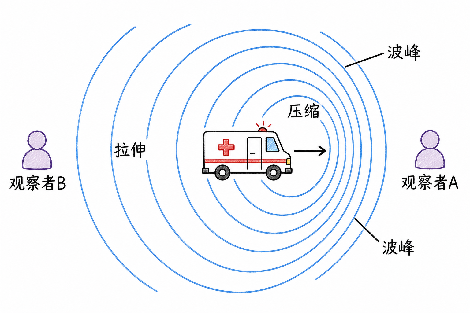
The entry point is still the Doppler effect. When you stand by the road and hear an ambulance approaching, the sound becomes higher-pitched; after it passes, the sound becomes lower. Radar sees a similar frequency shift in electromagnetic waves. Velocity measurement connects three things: why the frequency shift occurs, how to measure it, and why in pulse radar it manifests as phase rotation within the same range bin.
Starting with Sound Frequency Changes
You're standing by the road, an ambulance drives toward you from a distance, and the siren sounds higher-pitched; after the vehicle passes, the sound becomes lower. Everyone has heard this phenomenon, and it has a specific name:Doppler effect. When there is relative motion between the source and observer, the frequency received by the observer changes.
First build intuition with sound. Suppose the ambulance emits a sound at $f_0=1000\,Hz$ when stationary, and the speed of sound is approximately $v_s=340\,m/s$. This means 1000 wave crests are emitted from the speaker per second and are uniformly distributed in space. When the ambulance is stationary, the distance between adjacent wave crests is
If the ambulance moves toward the observer at $v=30\,m/s$, the speaker still emits 1000 wave crests per second, but when the next crest is emitted, the vehicle has already moved forward some distance. The spacing between crests in front is compressed, and as you stand still by the road, more crests pass you per unit time. The frequency received by the observer is approximately
The frequency increases, making the sound higher-pitched. If the ambulance moves away from the observer, the crest spacing is stretched, and the received frequency becomes
The frequency decreases, making the sound lower-pitched.
Radar transmits electromagnetic waves, not sound waves. The difference is that electromagnetic waves propagate at the speed of light $c\approx3\times10^8\,m/s$, and radar echoes undergo a two-way path from radar to target and back. When the target moves toward the radar, the echo frequency increases; when the target moves away, the echo frequency decreases.
In radar velocity measurement, typically only the low-speed approximation is needed. For a target with radial velocity $v_r$, transmit frequency $f_0$, and wavelength $\lambda=c/f_0$, the Doppler frequency shift can be written as
Conversely, after measuring the Doppler shift $f_d$, the radial velocity is
The factor of $2$ here comes from two-way propagation. The electromagnetic wave is affected by target motion once on the outbound path and once on the return path, so the radar Doppler shift is approximately twice that of the single-path case.
Radar Measures Radial Velocity
The $v_r$ in the formula represents the velocity component of the target along the radar line-of-sight direction; it only takes the portion of the true velocity projected onto the line of sight. If the target's true velocity is $v$ and the angle between its motion direction and the radar line of sight is $\theta$, then
This book adopts the convention: when the target approaches the radar, radial velocity $v_r$ is positive and Doppler shift $f_d$ is also positive; when the target recedes, both are negative. Different textbooks and systems may use opposite conventions, so check the sign convention before reading formulas.
When the target flies directly toward the radar, $\theta=0$ and the radial velocity equals the true velocity. When the target flies tangentially past the radar, $\theta=90^\circ$ and the radial velocity approaches 0—even if it's moving fast, the Doppler shift is very small.
If you want to fool a Doppler-only radar, you can circle around it. The velocity direction is always approximately tangential, so the radial velocity approaches 0; the target is certainly moving, but it's not approaching or receding along the radar line of sight, so in the Doppler dimension it looks more like stationary clutter.
Consider some orders of magnitude:
| Scenario | Radar Frequency / Wavelength | Radial Velocity | Doppler Shift |
|---|---|---|---|
| Traffic Radar | $f_0=24\,GHz$,$\lambda=0.0125\,m$ | $30\,m/s$ | $4.8\,kHz$ |
| Weather Radar | $f_0=3\,GHz$,$\lambda=0.1\,m$ | $10\,m/s$ | $200\,Hz$ |
| High-Speed Airborne Target | $f_0=10\,GHz$,$\lambda=0.03\,m$ | $600\,m/s$ | $40\,kHz$ |
The same velocity produces a larger Doppler shift at higher carrier frequencies. A larger shift is easier to measure, but the system must also be able to handle the corresponding frequency range.
5.2 Continuous Wave Velocity Measurement and Frequency Measurement
Obtaining the Beat Frequency Through Mixing
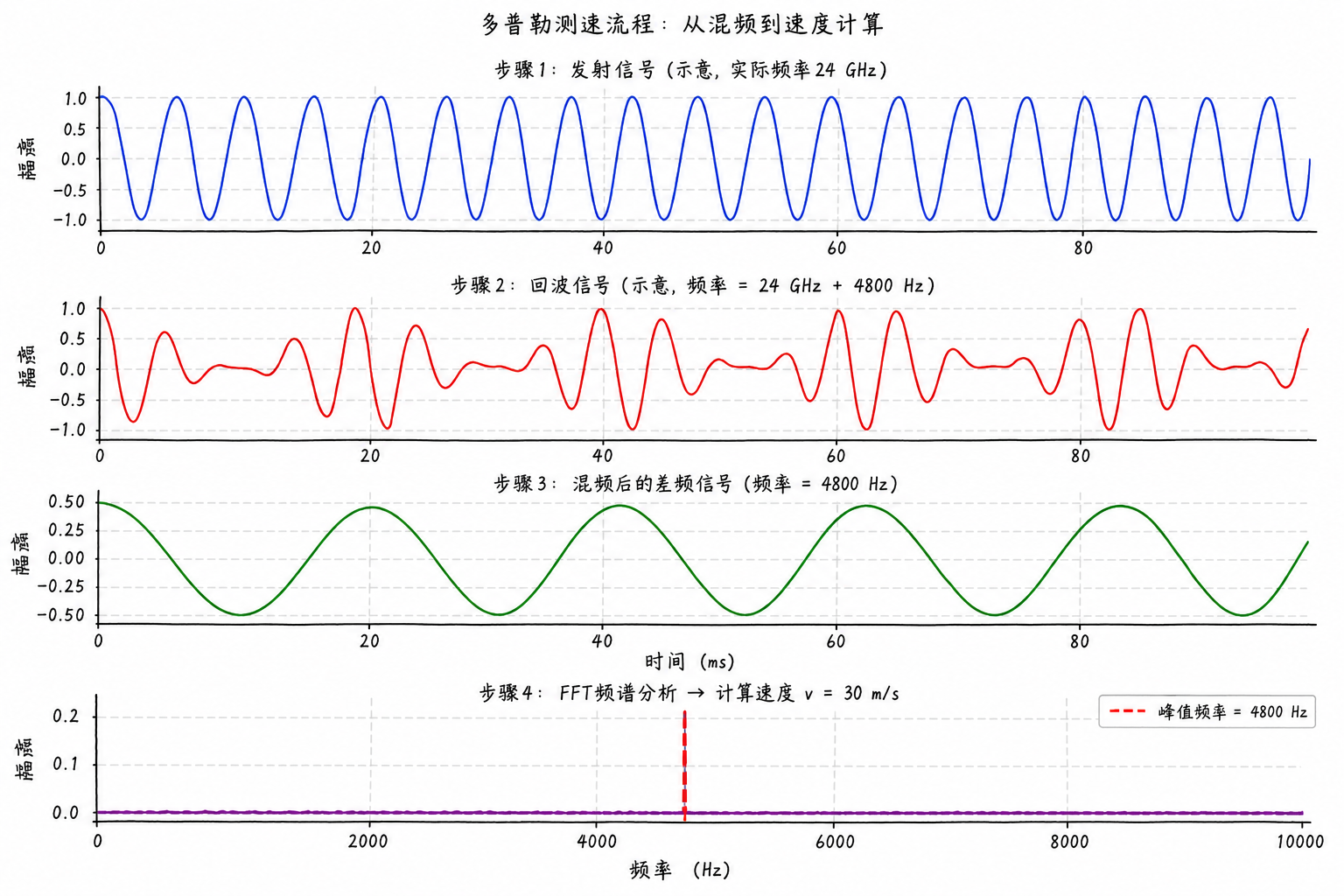
The simplest velocity measurement radar is the single-frequency continuous wave radar, referred to here as CW radar. It continuously transmits a single-frequency signal while receiving the target echo. If the target is moving, the echo frequency is shifted by $f_d$ relative to the transmitted frequency.
The formula shows that measuring $f_d$ yields the velocity. The challenge lies in accurately measuring this small frequency offset: the echo signal is very weak, the carrier frequency is often on the order of GHz, while the Doppler shift is typically only on the order of Hz to kHz.
Let the transmitted signal be
The received echo signal is approximately
If we perform FFT on the $24\,GHz$ raw RF signal, the sampling theorem requires a sampling rate of at least $48\,GHz$, making both hardware cost and data volume prohibitive. Receivers typically first multiply the transmitted signal with the received echo signal, a step called mixing:
The product contains two frequency components: one is the difference frequency $f_d$, typically on the order of Hz to kHz; the other is the sum frequency $2f_0+f_d$, still on the order of GHz. After a low-pass filter removes the sum frequency component, only the difference frequency signal remains
At this point, sampling and performing FFT allows measurement of $f_d$. Finally, substituting into
yields the radial velocity.
Practical receivers commonly use I/Q mixing to obtain a complex-valued difference frequency signal $e^{j2\pi f_dt}$. The complex difference frequency signal preserves positive and negative frequency information, allowing distinction between approaching and receding targets.
Limitations of Continuous Wave Radar
CW radar has a simple structure, suitable for scenarios focused solely on velocity measurement, such as handheld speed guns. Its limitation is also clear: the continuous wave is always transmitting, making it difficult for the receiver to determine range from "how late the echo arrives." Without modulation or other auxiliary designs, conventional CW radar cannot directly measure range using time delay like pulse radar.
Pulse radar processes differently. It first uses the range processing from Chapter 4 to determine which range bin the target falls into, then observes the complex-valued changes of that range bin across multiple pulses. In pulse radar, velocity information manifests as phase rotation in slow time.
| Waveform Type | Where Velocity Information Resides | Primary Processing Operation | Direct Range Measurement Capability |
|---|---|---|---|
| Single-frequency CW Radar | Beat frequency signal after mixing | FFT on beat frequency signal | Cannot measure range directly |
| Pulse-Doppler Radar | Slow-time phase of the same range bin | FFT along pulse index | Range measurable via time delay |
| FMCW Radar | Combined beat frequency and Doppler effect | 2D processing in fast time / slow time | Range measurable, but via different path |
Here CW specifically refers to unmodulated single-frequency continuous wave; although FMCW also transmits continuously, its frequency sweeps, making both range and velocity processing paths different—it cannot be conflated with single-frequency CW beat frequency velocity formulas.
5.3 Pulse-to-Pulse Phase and Slow-Time FFT
Focusing on a Single Range Bin
The previous section primarily discussed velocity measurement from the perspective of single-frequency CW radar: first mixing the high-frequency echo down to low frequency, then calculating velocity from the frequency offset. In pulse radar, velocity information is embodied in the phase change between adjacent pulses.
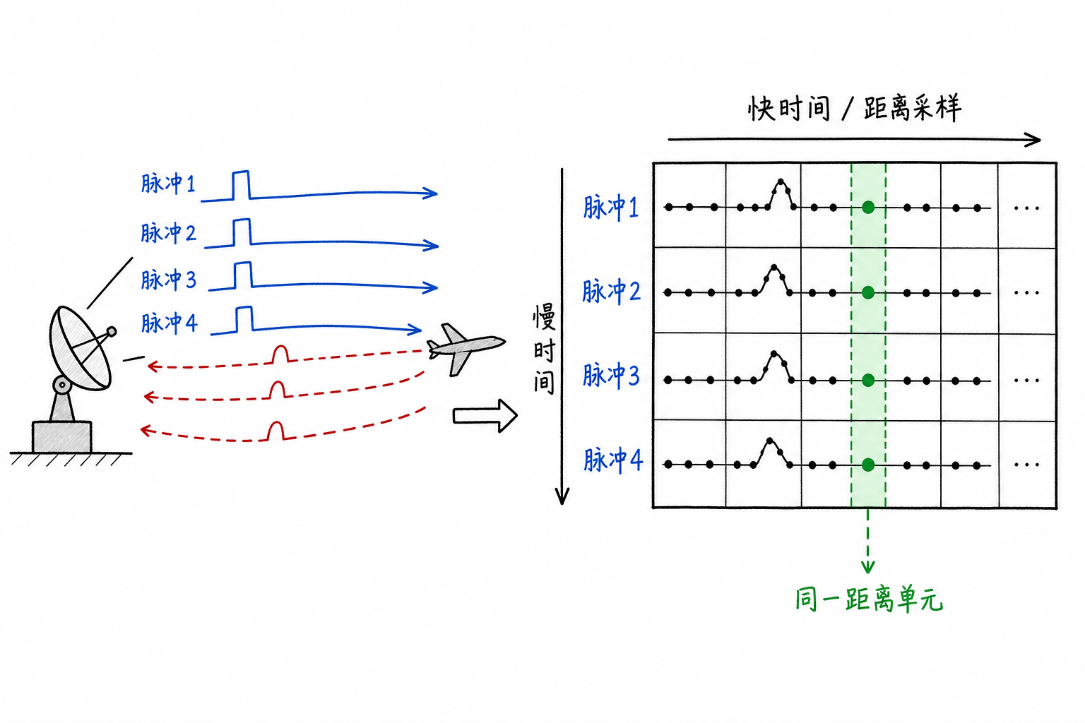
Chapter 4 already obtained the range profile. For a single pulse, the horizontal axis of the range profile is the range bin, and the peak position corresponds to the target range. Looking at just this one pulse, you can at most tell whether there is a strong echo in a certain range bin, but it's difficult to determine whether it's stationary, approaching, or receding. Now, by transmitting $N$ pulses consecutively, with each pulse undergoing range compression, we obtain $N$ range profiles.
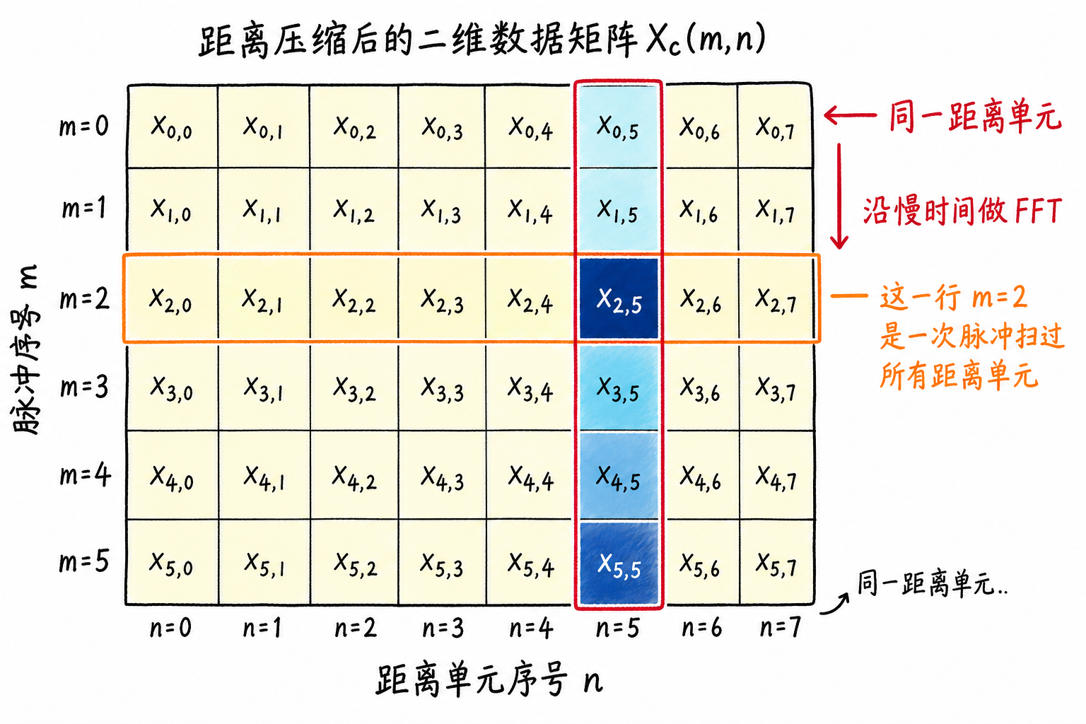
By arranging these range profiles according to pulse number, we get a two-dimensional matrix. The horizontal direction is the range bins after fast-time processing, and the vertical direction is the pulse number, also called slow time. If a target falls in the $n_0$-th range bin, we fix this column and extract
Here $X_c(m,n)$ represents the complex value of the $n$-th range bin after range compression of the $m$-th pulse. $z[m]$ is a sequence of complex samples along the slow-time direction for the same range bin.
Fast time is the sampling axis within a single pulse, with typically very short sampling intervals; slow time is the sampling axis between pulses, with a sampling interval equal to the PRI $T_r$. The "fast" and "slow" in the names refer precisely to the difference between these two sampling intervals. Figure 5.3 places these two sampling axes in the same matrix.
This can be compared to taking photographs: one photo can show where a person is standing, but only a series of photos taken at fixed time intervals can reveal whether they are continuously moving. If the target is stationary, ideally the phase variation of this sequence of complex numbers is very small; if the target is moving, from one pulse to the next, the target range changes slightly, the round-trip path changes accordingly, and the phase will rotate steadily with pulse number.
Let the interval between adjacent pulses be $T_r$. When the target radial velocity is $v_r$, the movement within one PRI is
The round-trip path change is
Since the electromagnetic wave advances the phase by $2\pi$ for every wavelength $\lambda$ traveled, the phase difference between adjacent pulses is
Using $f_d=2v_r/\lambda$, this can be written as
This equation connects velocity, Doppler frequency, and inter-pulse phase difference: the greater the target velocity, the faster the phase rotates in the same range bin.
From Phase Difference to Slow-Time FFT
If we only look at two adjacent pulses, we can also estimate velocity from the phase difference:
Since velocity can be calculated from just two pulses, why do we need FFT? Because two pulses give only one phase difference measurement, and with even slight noise, the estimate will fluctuate. When multiple pulses are combined, we can observe the entire sequence of phase variations; if there are two targets with different velocities in the same range bin, they may also separate in the frequency domain.
The slow-time sequence can be written in complex exponential form:
where $A$ is the amplitude and $\phi_0$ is the initial phase. It belongs to the same class of objects as the sinusoidal/complex exponential signals in Chapter 2, except the sampling interval is now the PRI $T_r$.
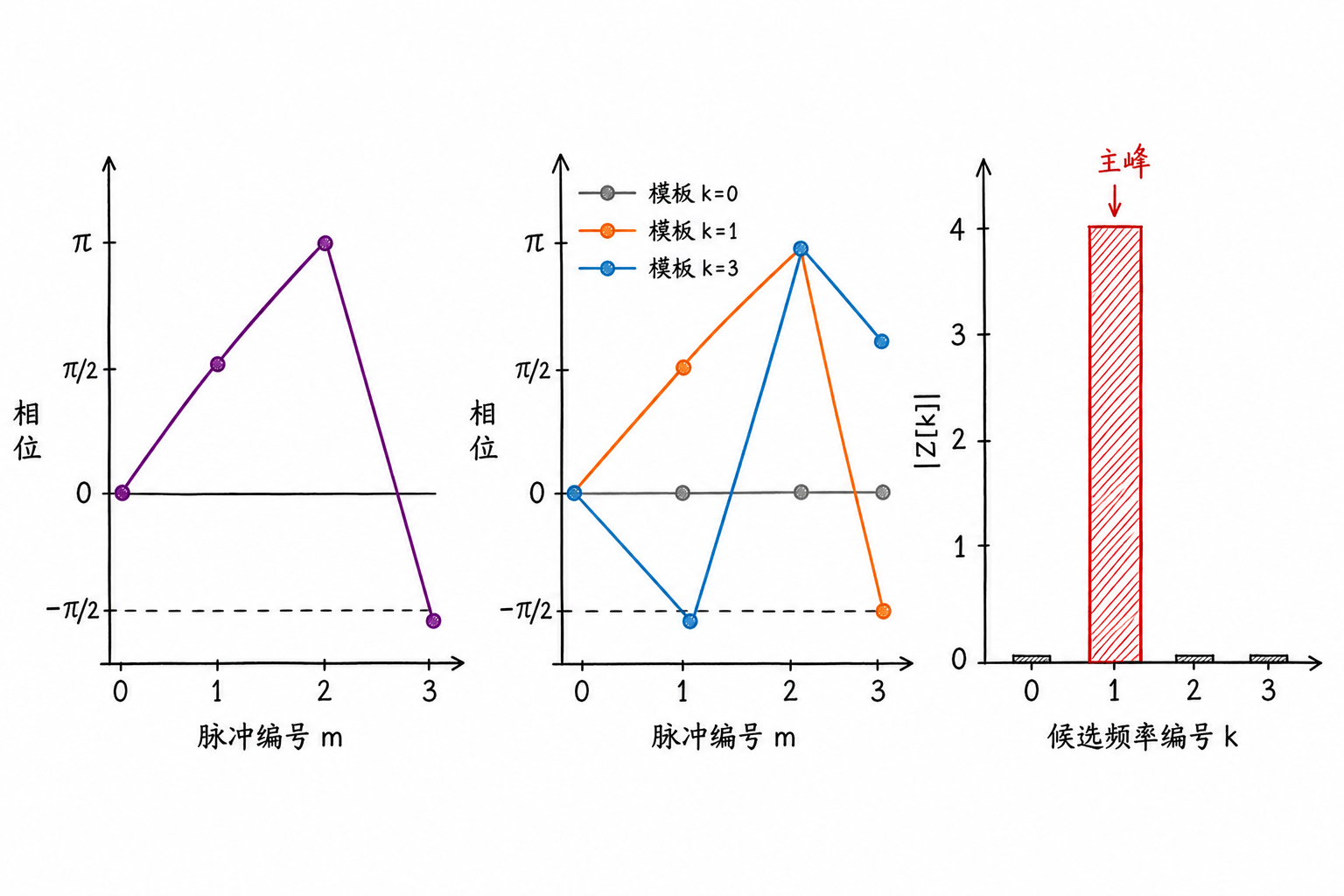
Let's use a 4-pulse example to see what the FFT does. Suppose a target's radial velocity creates an inter-pulse phase difference of exactly $90^\circ$. After fixing that range bin, the complex samples across4 consecutive pulses might be
The phases of these 4 complex numbers are sequentially
With each subsequent pulse, the phase advances by $90^\circ$. Performing a DFT on these 4 points:
First look at $k=1$:
The phase variation rate of the template $e^{-j2\pi m/4}$ exactly cancels the phase variation of the samples, so all four terms add in the same direction, resulting in maximum amplitude.
Now consider $k=0$:
$k=0$ corresponds to a template with no phase rotation, which doesn't match this sample sequence and cancels out after accumulation.
The FFT peak position corresponds to the slow-time phase rotation rate. The Doppler frequency for the $k$-th bin is
If $N=4$ and $T_r=1\,ms$, then $\text{PRF}=1000\,Hz$. The above $k=1$ corresponds to
We can also verify in reverse: a Doppler frequency of $250\,Hz$ with pulse interval $T_r=1\,ms$ gives a phase difference between adjacent pulses of
This exactly corresponds to the sequence $1,j,-1,-j$ from before. If the radar operates at $10\,GHz$ with wavelength $\lambda=0.03\,m$, the velocity is
In this way, the inter-pulse phase change is converted to Doppler frequency, which is then converted to radial velocity.
5.4 MTD and Range-Doppler Maps
Slow-Time FFT for Each Range Bin
The previous section focused on a single range bin. In practice, radar must process the entire two-dimensional data matrix: horizontally distinguishing different ranges, and vertically observing changes in the same range bin across multiple pulses.
After transmitting $N$ pulses, the range-compressed output can be arranged into a complex matrix:
where $m$ is the pulse index and $n$ is the range bin. For each fixed $n$, performing an FFT along the $m$ direction yields the Doppler distribution for that range bin. After processing all range bins, the result is still a two-dimensional map, but the vertical axis has changed from 'pulse index' to 'Doppler frequency' or 'velocity'.
This processing is commonly called MTD(Moving Target Detection). In the introductory context of this book, MTD can be understood as: after range processing, performing a slow-time FFT on each range bin separately to separate moving targets by Doppler frequency.
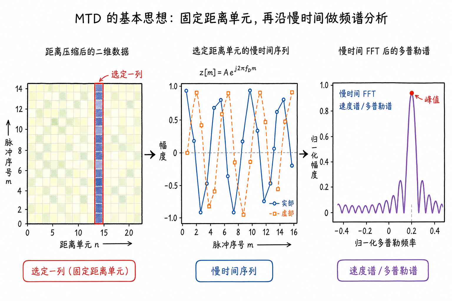
The left side of Figure 5.6 shows the range-compressed matrix. After selecting a specific range bin, extract a column of complex samples along slow time; performing an FFT on this column yields the velocity spectrum at that range. Repeating this operation for all columns produces the range-velocity map.
Reading Range-Doppler Maps
The range-velocity map is also called a range-Doppler map. The horizontal axis represents range, the vertical axis represents Doppler frequency or converted radial velocity, and each pixel on the map represents the response intensity of a specific range-velocity cell.
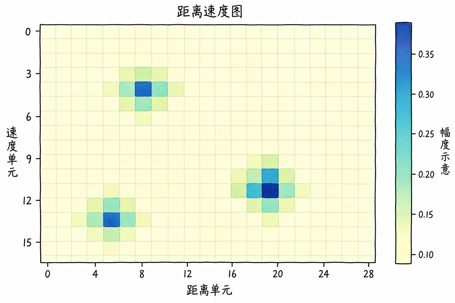
When reading such maps, first look at the horizontal position of bright spots to determine the possible range of a target; then look at the vertical position to determine the possible radial velocity. If a bright spot is located near $15\,km$ and $+30\,m/s$, it indicates a strong response in that range-velocity cell: the target may be at 15 km and approaching the radar at approximately $30\,m/s$ radial velocity.
It's important to distinguish between 'response' and 'target'. Bright spots on the range-velocity map are only candidate responses in the processing results, which may come from targets, but also from noise, clutter, or sidelobe leakage. Whether the radar reports it as a target requires threshold and CFAR detection in Chapter 6; if multiple adjacent bright spots appear near a target, they must be consolidated into a single target plot through plot clustering after detection.
MTD has another advantage: stationary ground clutter, buildings, and other clutter are typically concentrated near zero Doppler, appearing as a bright stripe near zero velocity in the plot. Moving targets with significant radial velocity appear in non-zero velocity bins. The velocity dimension thus provides a handle for separating moving targets from stationary clutter.
5.5 Velocity Resolution, Ambiguity, and PRF Tradeoffs
CPI and Velocity Resolution
The frequency spacing of the slow-time FFT is
$NT_r$ is the total duration of this coherent processing, called the CPI(Coherent Processing Interval, CPI):
Therefore
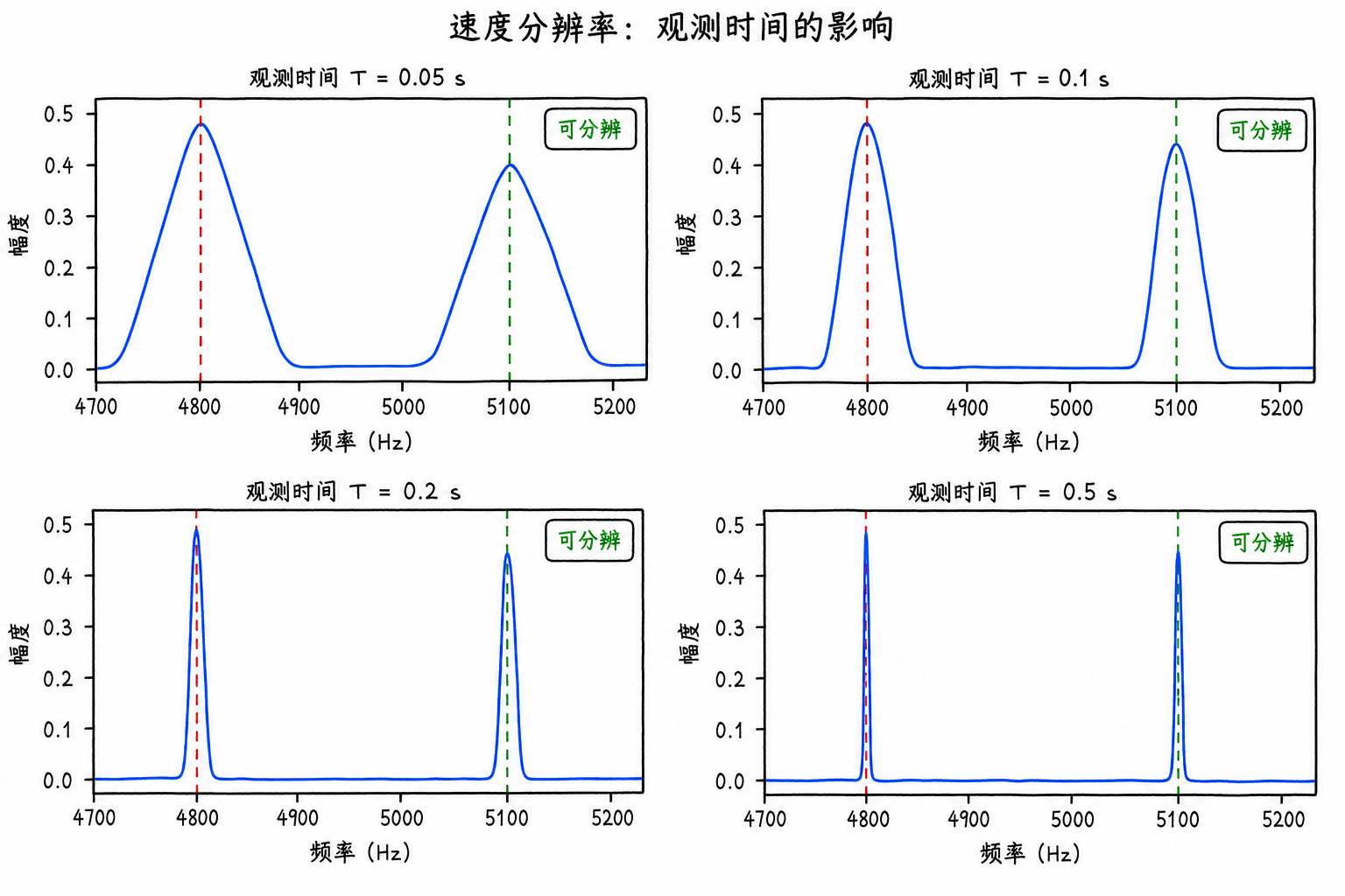
From $v_r=\lambda f_d/2$, the velocity resolution is
This describes whether two targets with similar velocities can be separated on the velocity axis. The longer the CPI, the denser the FFT bins, and the finer the velocity resolution.
For example, with $\lambda=0.03\,m$ and $T_{\text{CPI}}=0.1\,s$, we get
To improve the velocity resolution to $0.05\,m/s$, we need
CPI cannot be extended indefinitely. When the target accelerates, maneuvers, or migrates across range cells, the slow-time sequence no longer behaves like a stable complex exponential; the radar must also maintain a data update rate and cannot wait indefinitely for finer velocity bins.
PRF and Maximum Unambiguous Velocity
The slow-time sampling interval is $T_r$, and the sampling rate is $\text{PRF}=1/T_r$. For complex I/Q slow-time sequences, the unambiguous frequency range of the FFT is typically written as
Beyond this range, Doppler frequencies fold back, creating velocity ambiguity. Substituting $f_d=2v_r/\lambda$ into this range gives
Multiplying both sides by $\lambda/2$ yields
This is the maximum unambiguous velocity convention adopted in this book.
For example, with $\lambda=0.03\,m$ and $\text{PRF}=2000\,Hz$, we get
If the target's radial velocity exceeds this range, the FFT peak folds to another velocity position. A high-speed approaching target may be displayed as a low-speed target, or even displayed in the receding direction.
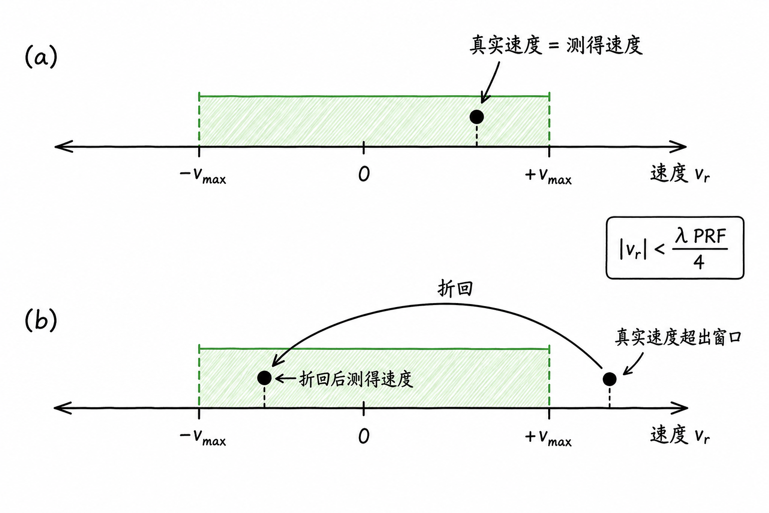
Some textbooks write $v_{\max}=\lambda\text{PRF}/2$. This commonly arises from different conventions for spectral range, distinguishing positive and negative directions, or single-sided/double-sided display. This book uses complex I/Q double-sided spectrum, hence the denominator is 4.
Range-Velocity Tradeoff in PRF
PRF appears to be just a transmit parameter, but it constrains both range and velocity dimensions. Chapter 3 already explained that the unambiguous range for pulse radar is approximately
The higher the PRF, the shorter the interval between adjacent pulses, and the next pulse is transmitted sooner; echoes from distant targets may return after the next pulse is transmitted, causing range ambiguity. On the other hand, the higher the PRF, the higher the slow-time sampling rate and the larger the maximum unambiguous velocity.
| Parameter Change | Benefit | Cost |
|---|---|---|
| Increase PRF | Maximum unambiguous velocity increases | Unambiguous range decreases |
| Decrease PRF | Unambiguous range increases | Maximum unambiguous velocity decreases |
| Extend CPI | Velocity resolution becomes finer | Data update slows down, target maneuver effects become more pronounced |
| Shorten wavelength | Same velocity produces larger Doppler shift | Unambiguous velocity range decreases at fixed PRF, and hardware precision and propagation environment requirements become higher |
Velocity resolution is primarily determined by CPI; do not confuse it with the effect of PRF. If CPI is fixed, changing PRF mainly affects the measurable velocity range and unambiguous range; if the pulse count $N$ is fixed, increasing PRF shortens the CPI, making velocity resolution coarser instead.
This PRF tradeoff between range and velocity is commonly called the Doppler dilemma in radar textbooks. Practical systems use multiple PRFs, staggered PRFs, or other ambiguity resolution methods; this book does not cover these algorithms in detail.
5.6 Practical Applications
Speed Gun
Traffic speed guns typically use CW systems, operating in bands such as 24 GHz or 35 GHz. They continuously transmit single-frequency electromagnetic waves, receive vehicle echoes and mix them with the local oscillator to obtain the Doppler difference frequency; then perform FFT on the difference frequency signal, locate the spectral peak, and convert it to vehicle speed.
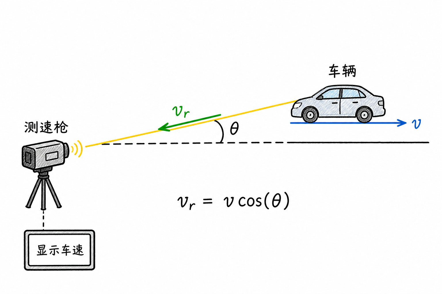
Speed guns only need to measure vehicle speed, not necessarily distance, so the CW system is sufficient. They are also affected by angle: when the angle between the speed gun and the vehicle's direction of motion is $\theta$, the measured value is $v\cos\theta$. The greater the angle deviation, the lower the displayed speed.
Weather Radar
Weather radars face numerous scatterers such as raindrops, snowflakes, and hail. They need to determine not only wind speed but also the range and azimuth of these returns, so pulse-Doppler systems are commonly used.
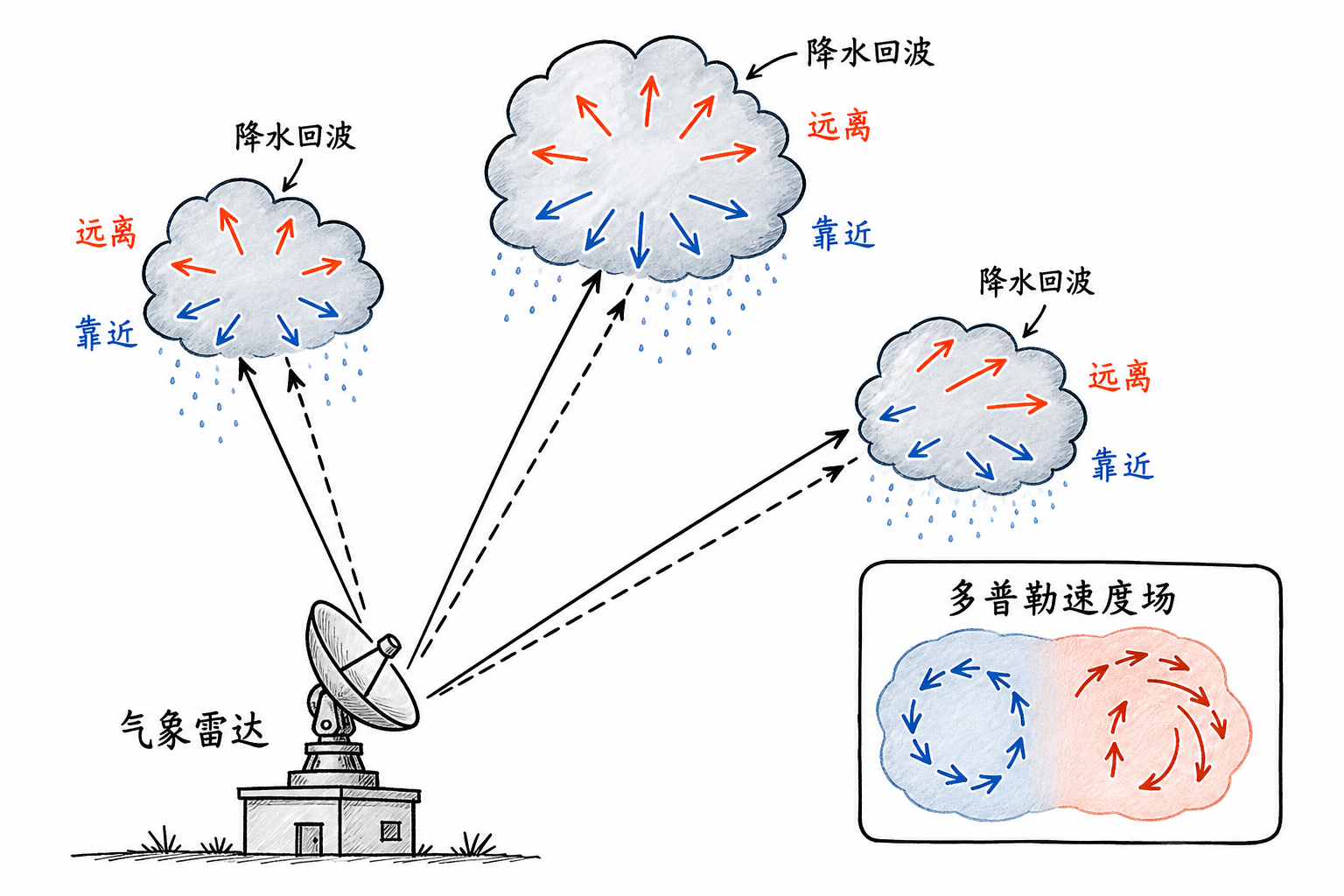
Weather radars first use echo delay to determine the location of precipitation regions, then estimate radial velocity from phase changes between adjacent pulses. If a region shows strong velocities alternating between positive and negative at adjacent locations, this may indicate local rotational structures; phenomena such as wind shear and strong convection are also reflected in the Doppler velocity field.
Weather radars typically require large unambiguous range, so PRF cannot be arbitrarily increased; however, low PRF easily introduces velocity ambiguity. This is why velocity dealiasing is frequently required in weather radar processing.
Automotive Radar
Modern automotive radars typically operate in the 77 GHz band and are commonly used for adaptive cruise control, automatic emergency braking, blind spot monitoring, and other functions. They must measure both range and velocity while handling multiple targets.
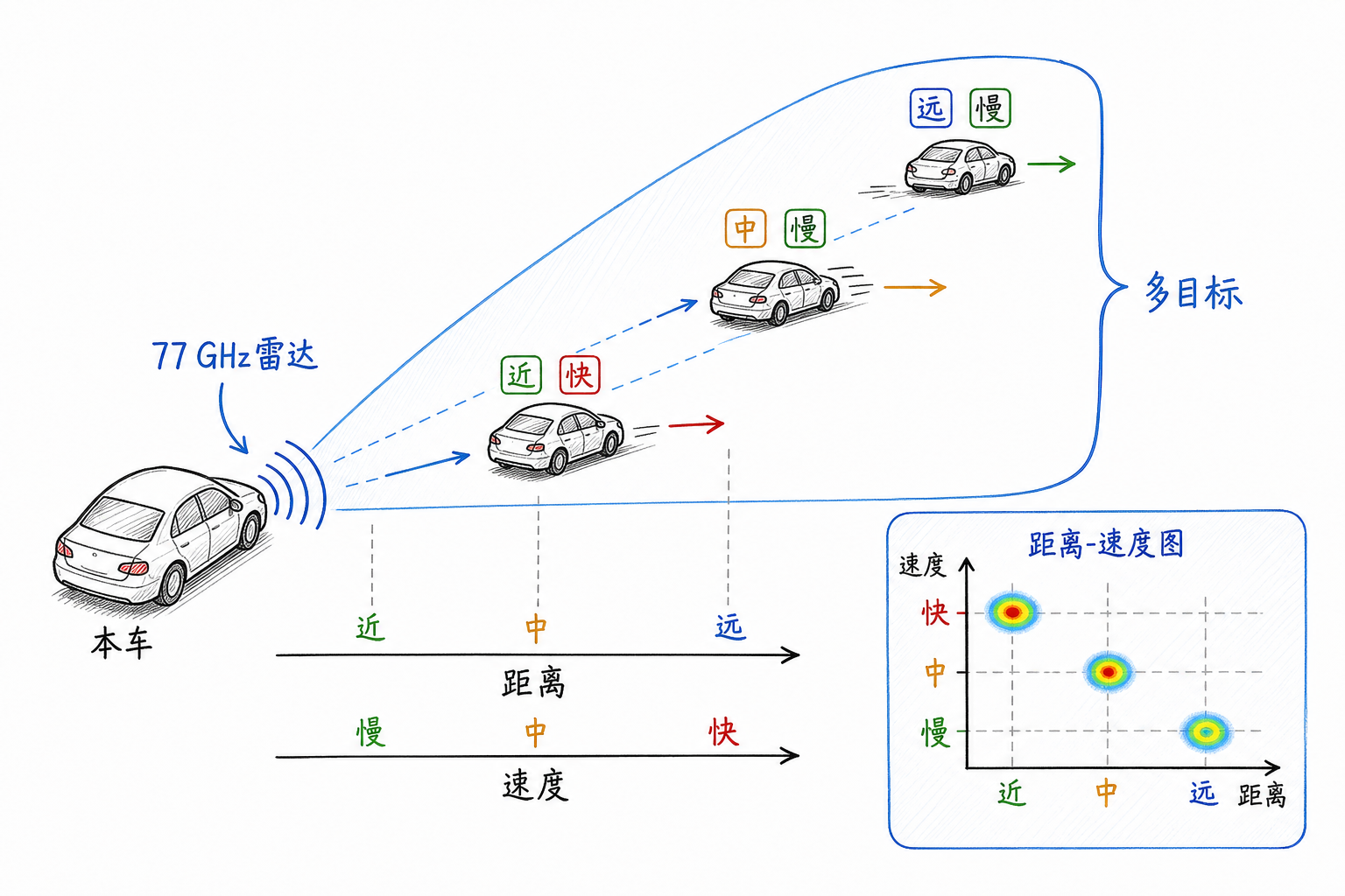
Automotive radars commonly use FMCW systems. FMCW also utilizes Doppler information, but the extraction paths for range and velocity differ from the pulse-Doppler processing discussed earlier: it generates beat frequencies through linear frequency sweeps, with range and velocity jointly affecting the mixed signal, requiring FMCW's two-dimensional processing methods to separate them. We treat this as an application boundary and do not mix FMCW formulas into this pulse-Doppler pathway.
Issues in Real Systems
Clutter concentrates near zero Doppler. Strong returns from ground, buildings, sea surface, etc., may be stronger than the target itself. One task of MTI/MTD is to suppress these low-velocity or zero-velocity backgrounds.
Multiple targets will superimpose on each other. If two targets with different velocities exist in the same range cell, slow-time FFT may separate them; if their velocity difference is smaller than the velocity resolution, they will still fall within the same Doppler bin vicinity.
High-speed targets may experience velocity ambiguity. Increasing PRF can expand the unambiguous velocity range but sacrifices unambiguous range. Engineering design often involves trade-offs among these constraints.
5.7 Exercises
Exercise 1: Basic Doppler Conversion
A radar operating at $10\,GHz$ measures a Doppler frequency shift of $3000\,Hz$ for a target. What is the target's radial velocity?
Solution: First find the wavelength
From the velocity conversion formula
we obtain
Converting to km/h, approximately
Exercise 2: Angular Error in Speed Guns
A traffic police officer uses a $24\,GHz$ speed gun to measure vehicle speed. The speed gun makes a $30^\circ$ angle with the vehicle's direction of motion, and the measured Doppler frequency shift is $4157\,Hz$. What is the vehicle's true speed?
Solution: $24\,GHz$ corresponds to wavelength
The measured radial velocity is
Since
Therefore
which is approximately $108\,km/h$.
Exercise 3: CPI and Velocity Resolution
A radar has a wavelength of $0.03\,m$ and CPI of $0.1\,s$. What is the velocity resolution? If a velocity resolution of $0.05\,m/s$ is desired, how long should the CPI be?
Solution:
If $\Delta v=0.05\,m/s$ is required, then
Exercise 4: Maximum Unambiguous Velocity
A pulse Doppler radar has a wavelength of $0.03\,m$ and PRF of $2000\,Hz$. Using the complex I/Q two-sided spectrum convention, what is the maximum unambiguous velocity?
Solution:
If the target radial velocity exceeds this range, the slow-time spectrum will fold, and the velocity reading may appear at an incorrect location.
Exercise 5: Reading Range-Doppler Maps
A range-velocity map has a bright spot at $15\,km$, $+30\,m/s$. What does this bright spot indicate? What needs to be done next?
Solution: This bright spot indicates a strong echo response in the cell at range $15\,km$ and radial velocity approximately $+30\,m/s$. According to the convention in this book, positive velocity indicates the target is approaching the radar.
However, it is not yet a final target report. The range-velocity map only provides candidate responses; a threshold or CFAR must be used to determine if it exceeds the surrounding background before deciding whether to report it as a target.